Journal of Biomedical Engineering and Biosciences (JBEB)
ISSN: 2564-4998

Volume 7 - Year 2020 - Pages 31-40
DOI: 10.11159/jbeb.2020.004
Sensitivity Analysis of a Phenomenological Thrombosis Model and Growth Rate Characterisation
Gian Marco Melito1, Alireza Jafarinia2, Thomas Hochrainer2, Katrin Ellermann1
1University of Technology Graz, Institute of Mechanics
Kopernikusgasse 24/IV, Graz, Austria 8010
gmelito@tugraz.at; ellermann@tugraz.at
2University of Technology Graz, Institute of Strength of Materials
Kopernikusgasse 24/I, Graz, Austria 8010
alireza.jafarinia@tugraz.at; hochrainer@tugraz.at
Abstract - Aortic dissection is a severe cardiovascular disease caused by the occurrence of a tear in the aortic wall. As a result, the blood penetrates the wall and makes a new blood channel called the false lumen. The haemodynamic conditions in the false lumen may contribute to the formation of thrombi, which influence the patient's diagnosis and outcomes. In this study, the focus is on a haemodynamic-based model of thrombus formation. Since the model construction entails uncertainties in the model parameters, a variance-based sensitivity analysis is performed. Thrombus formation at a backward-facing step is considered as a benchmark for the numerical simulations and sensitivity analysis. This geometry is capable of representing the main contributions of the model in thrombus formation. The study aims at improving the understanding of the model's structure and at preparing model simplifications to enable efficient patient-specific simulations in the future. A polynomial chaos expansion is employed as a surrogate model, from which the quantitative sensitivity indices are derived. In this study, nine model parameters are selected, whose proper values are not well known. The model responses taken into account are the maximum volume fraction of thrombus, its time development, and the thrombus growth rate. The results show that the model lends itself to model reduction since some of the model parameters show little to no influence on the model's outputs. A threshold value related to the concentration of bounded platelets and the bounded platelets reaction rate are identified as the key input parameters dominating the thrombus model predictions in the current geometry. Furthermore, the introduced thrombus characteristic growth time is driven by both the aforementioned variables.
Keywords: Aortic Dissection, Thrombus Formation, Global Sensitivity Analysis, Backwards-Facing Step.
© Copyright 2020 Authors This is an Open Access article published under the Creative Commons Attribution License terms. Unrestricted use, distribution, and reproduction in any medium are permitted, provided the original work is properly cited.
Date Received: 2020-10-20
Date Accepted: 2020-11-10
Date Published: 2020-12-09
1. Introduction
Aortic dissection (AD) is a disease that develops a second volume, called false lumen (FL), in the aorta. AD is classified as type A when it initiates in the ascending thoracic aorta, type B when the initial tear in the aortic wall is in the descending thoracic aorta (Stanford Classification System). Type B aortic dissection (TBAD) is a severe disease associated with high mortality, which may also lead to complications such as aortic aneurysm, rupture or malperfusion syndromes [1]. In the current study, the focus is on TBAD and the role of thrombosis in the false lumen.
The haemodynamic conditions in the FL, including flow disturbance, recirculations, and significant variability in the wall shear stress (WSS) presumably promote the formation and growth of thrombi [2]. In [3], it is shown that partial thrombosis is associated with a higher mortality rate, whereas complete thrombosis of the FL improves patients' prognosis [4], [5]. Up to now, it is not entirely clear what circumstances favour thrombosis following aortic dissection. Thrombus formation models may play a vital role in the analysis of haemodynamics in cardiovascular environments.
In [2] and [6], a haemodynamic-based model capable of predicting false lumen thrombosis in TBAD is developed. However, because the model is mostly phenomenological, the parameters of the model may not be determined from chemical or biological characteristics of the blood. Instead, the parameters will usually be obtained from inverse modelling, i.e. fitting to measured data. However, suitable time-resolved data of thrombus-formation is very sparse, which is why it is of vital importance to narrow down the number of model parameters. A global sensitivity analysis is suggested to understand the influence of the parameters [7].
The model performs well in predicting the location of thrombus formation; however, it is unable to reproduce the growth rate as observed in in-vivo and in-vitro studies. More insight into the model parameters and their role in thrombus growth is needed to bridge the gap between numerical simulations and real-life studies. This paper identifies the most critical parameters for the thrombus growth model, and further analysis of the thrombus characteristic growth time indicates the parameters that could accelerate or inhibit the process of thrombus formation.
The paper is structured as follows: the thrombus formation model is exposed in Section 2, the theory of sensitivity analysis is explained in Section 3, while its application to the computational model is in Section 3.2. Results of the analysis and the conclusions are exposed in Sections 4 and 5, respectively.
2. Thrombus Formation and Growth
In this study, the thrombus
formation model developed in [2] is used. It is a haemodynamic-based model in
which the thrombus forms and grows mainly in areas where low shear stress and
high residence time are measured. The model consists of the following equations,
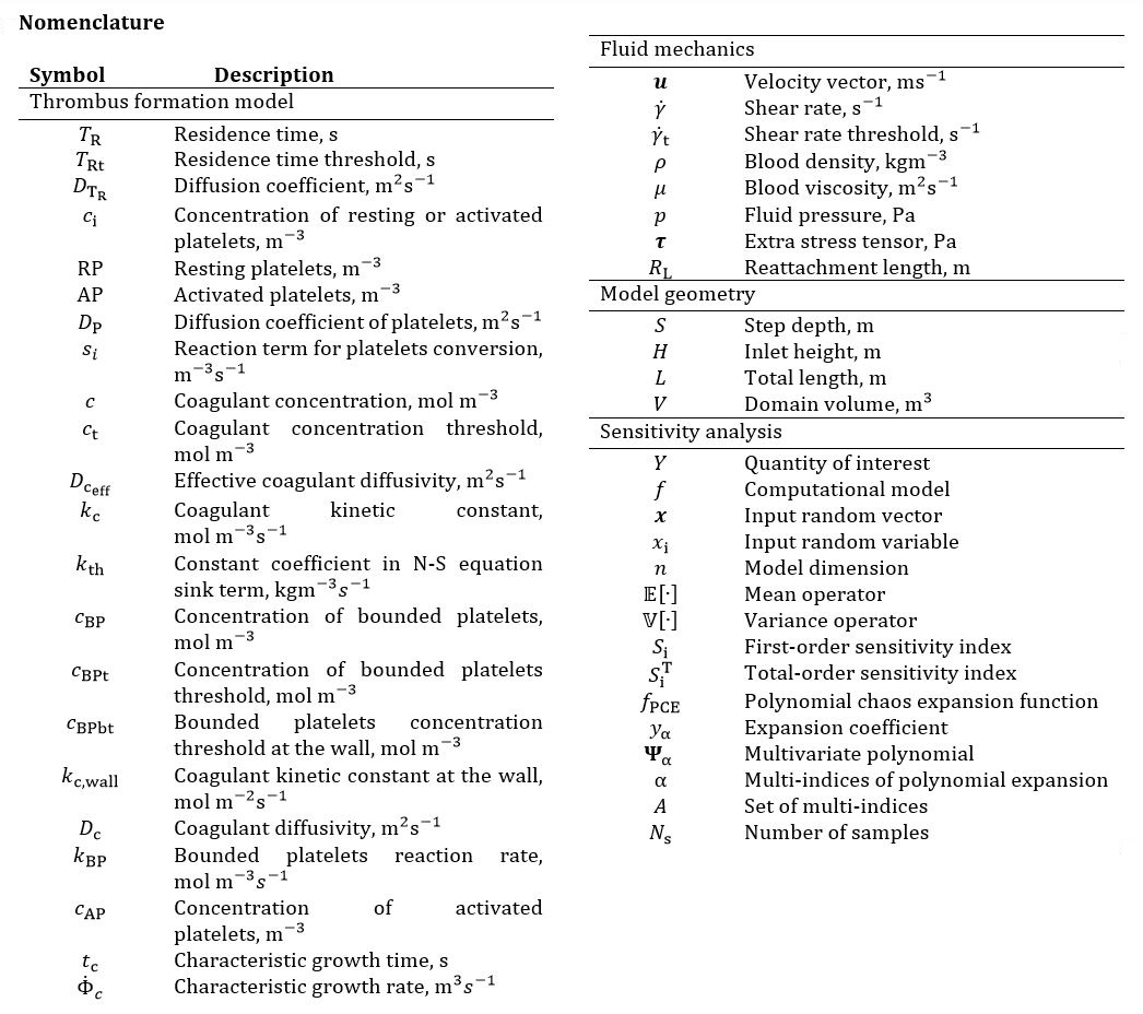
which are coupled with Navier-Stokes equations. The residence time ![]() is a field quantity, which obeys
the following evolution law,
is a field quantity, which obeys
the following evolution law,
where ![]() denotes
the velocity vector, and
denotes
the velocity vector, and ![]() is a diffusion coefficient. High
is a diffusion coefficient. High ![]() marks areas where platelets spend
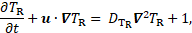
more time [2]. The transport equation for the concentration
marks areas where platelets spend
more time [2]. The transport equation for the concentration ![]() of resting or activated platelets
(RP or AP, resp.) is
of resting or activated platelets
(RP or AP, resp.) is
Here, ![]() denotes the diffusion coefficient
of platelets, which is the same for resting and activated platelets.
Furthermore,
denotes the diffusion coefficient
of platelets, which is the same for resting and activated platelets.
Furthermore, ![]() denote reaction terms for the
conversion of resting to activated platelets [2].
denote reaction terms for the
conversion of resting to activated platelets [2].
The so-called coagulant
concentration ![]() accounts
for the lumped effect of all underlying biochemical reactions in the
coagulation cascade [2]. In low shear rate areas, there is a production of
coagulant at the wall based on the conditions specified on the boundary, compare
Eq. (5). This modified boundary condition for the flux of coagulant is taken
from [6] for the backwards-facing step. The diffusion-reaction equation for the
coagulant is
accounts
for the lumped effect of all underlying biochemical reactions in the
coagulation cascade [2]. In low shear rate areas, there is a production of
coagulant at the wall based on the conditions specified on the boundary, compare
Eq. (5). This modified boundary condition for the flux of coagulant is taken
from [6] for the backwards-facing step. The diffusion-reaction equation for the
coagulant is

where ![]() is the coagulant kinetic constant,
is the coagulant kinetic constant, ![]() is
the shear rate. Furthermore,
is
the shear rate. Furthermore,
where the
subscript ![]() denotes
the threshold values, and
denotes
the threshold values, and
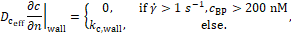
The effective coagulant diffusivity ![]() is proportional to the coagulant
diffusivity
is proportional to the coagulant
diffusivity ![]() ,
,

Finally, the rate of production of
bounded platelets concentration ![]() is given by
is given by
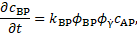
where
Here, ![]() denotes the bounded platelets
reaction rate and
denotes the bounded platelets
reaction rate and ![]() is the activated platelets
concentration. The Navier-Stokes equation is modified to incorporate the
thrombus growth [2]
is the activated platelets
concentration. The Navier-Stokes equation is modified to incorporate the
thrombus growth [2]
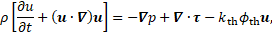
where ![]() denotes
the blood density,
denotes
the blood density, ![]() the
pressure,
the
pressure, ![]() is
the extra stress tensor, and
is
the extra stress tensor, and
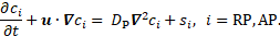
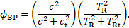
The quantity ![]() indicates local thrombosis as a
function of the bounded-platelets concentration
indicates local thrombosis as a
function of the bounded-platelets concentration ![]() and its threshold
and its threshold ![]() . Furthermore,
. Furthermore, ![]() is a coefficient with a
sufficiently high value to stop the flow where the thrombus is formed [2]. In
summary, the model controls the formation of thrombus based on shear stress,
residence time, the concentration of coagulant and platelets.
is a coefficient with a
sufficiently high value to stop the flow where the thrombus is formed [2]. In
summary, the model controls the formation of thrombus based on shear stress,
residence time, the concentration of coagulant and platelets.
3. Numerical Simulations
OpenFOAM software is used for
solving the blood flow and thrombus formation equations. The blockMesh
utility in OpenFOAM is used for generating a
structured hexahedral mesh. Blood is modelled as a Newtonian fluid. The
geometry is characterised by a step depth (![]() ) of 2.5 mm,
inlet height (
) of 2.5 mm,
inlet height (![]() ) of 7.5 mm and a total length (
) of 7.5 mm and a total length (![]() ) of 120 mm.
) of 120 mm.
3. 1. Initial and Boundary Conditions
For the inlet boundary condition of the velocity, a uniform velocity profile resulting in Reynolds number of 490 was imposed, with the no-slip condition for the walls. The pressure gradient is equal to zero on all the boundaries except the outlet, which is considered having a fixed value of zero.
As discussed in sections 2, there are five
equations to be solved for the thrombus formation model. For solving residence
time ![]() equation (Eq. 1), which is initially zero, the inlet
value of
equation (Eq. 1), which is initially zero, the inlet
value of ![]() is fixed to zero, and the normal gradient on
all the other boundaries is set to zero.
is fixed to zero, and the normal gradient on
all the other boundaries is set to zero.
Initial values of resting platelets RP and activated platelets AP in the blood are taken from [2]. The inlet values of RP and AP (Eq. 2) are fixed to their initial values. Zero normal gradients of AP and RP is imposed on all the other boundaries. For the coagulant equation (Eq. 3), the Neumann boundary condition discussed in section 2 is implemented for the walls, while a zero fixed value at the inlet and a zero normal gradient at the outlet are applied. Bounded platelets equation (Eq. 7) is solved with zero initial concentration of bounded platelets.
3. 2. Backward-facing step benchmark
The thrombus formation simulation starts at 12
seconds from the steady-state flow solution. A Reynolds number of 490 is chosen
to be consistent with in-vitro results in [8] and numerical simulations in [9].
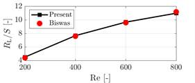
To test the performance of numerical simulations, the reattachment length ![]() at the back of the step for four Reynolds
numbers is compared to the numerical results of [10]. For this comparison, the
expansion ratio of
at the back of the step for four Reynolds
numbers is compared to the numerical results of [10]. For this comparison, the
expansion ratio of ![]() is adopted [10]. The Reynolds number
is adopted [10]. The Reynolds number ![]() is computed as
is computed as

where ![]() is inlet velocity,
is inlet velocity, ![]() is the hydraulic diameter and equal to
is the hydraulic diameter and equal to ![]() [10],
[10], ![]() is the blood density, and blood viscosity
is the blood density, and blood viscosity ![]() [9].
[9].
Figure 1 shows that the present results are in good agreement with the benchmark solutions [10]. Mesh and time-step sensitivity analysis resulted in 20,000 elements and a time-step of 0.005s.
3. 3. Thrombus formation model
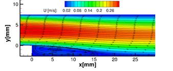
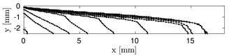
In Figure 2, the recirculation area behind the step is highlighted by the streamlines superposed on a density plot of the magnitude of the fluid velocity. The model predicts thrombus formation in the recirculation area behind the step which qualitatively matches with in-vitro results in [8] and numerical simulations in [9], see Figure 3.
4. Sensitivity analysis
Consider a quantity of interest ![]() of
computational model
of
computational model ![]() function of
an input random vector
function of
an input random vector ![]() of dimension
of dimension
![]() , i.e.
, i.e. ![]() . One of the most widely used technique in
global sensitivity analysis is the variance-based method, which quantifies the
connection between the variance of the model output
. One of the most widely used technique in
global sensitivity analysis is the variance-based method, which quantifies the
connection between the variance of the model output ![]() , given the
variability of its inputs
, given the
variability of its inputs ![]() . The sensitivity analysis may be employed for
model reduction, in that the non-influential variables of a computational model
may be considered constants. Furthermore, sensitivity analysis enables input
factor prioritisation, by ranking the parameters, to which the outcome is most
sensitive.
. The sensitivity analysis may be employed for
model reduction, in that the non-influential variables of a computational model
may be considered constants. Furthermore, sensitivity analysis enables input
factor prioritisation, by ranking the parameters, to which the outcome is most
sensitive.
A random variable ![]() is considered to be influential
(non-influential) to the model
is considered to be influential
(non-influential) to the model ![]() with output
with output ![]() if the
conditional variance
if the
conditional variance ![]() is larger (smaller) than the variance of the
quantity of interest
is larger (smaller) than the variance of the
quantity of interest ![]() , where
, where ![]() and
and ![]() represent the variance and the mean operators.
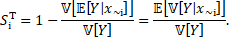
The first-order sensitivity index (or first-Sobol index) is defined as [11]
represent the variance and the mean operators.
The first-order sensitivity index (or first-Sobol index) is defined as [11]

The first-Sobol index represents the
contribution of the random variable ![]() , for
, for ![]() , to the change of the model output
, to the change of the model output ![]() .
.
The total-order sensitivity index (or total-Sobol index) is defined as
The total-Sobol index evaluates the total effect
of an input parameter, by accounting for the conditional variance of the
output, conditioning to all factors except the given one, ![]() .
.
The first-Sobol index identifies the level of influence of a single parameter on the output in the analysis, but it does not give information regarding the interaction of the parameter with other variables of the input space. It may be used for factor prioritisation, where a ranking of the parameters is produced. The rank indicates the level of influence on the model variation, and therefore it highlights the input uncertainty that needs to be removed. The total-order sensitivity index specifies the influence of the input parameter on the model output and the level of interaction with other input parameters. The total-order index is used for factor fixing. Here, the lower values are considered to decide which variable has no- or low-effect on the output. Such variables can be successively considered as model's constant.
4. 1. Polynomial Chaos Expansion
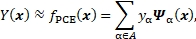
The Sobol indices are assessed from a polynomial chaos expansion (PCE) of the computational model [12].
PCE consists of the sum of
orthogonal, multivariate polynomials ![]() of increasing order up to some
maximal polynomial order
of increasing order up to some
maximal polynomial order ![]() [13].
The polynomials are multiplied by expansion coefficients
[13].
The polynomials are multiplied by expansion coefficients ![]() , which can be estimated with
different methods. The expansion is written as
, which can be estimated with
different methods. The expansion is written as
where ![]() is
a set of multi-indices α which refer to the degree of each polynomial with
respect to each input parameter. The multivariate polynomials
is
a set of multi-indices α which refer to the degree of each polynomial with
respect to each input parameter. The multivariate polynomials ![]() are defined as the product of
univariate polynomials of order
are defined as the product of
univariate polynomials of order ![]() , i.e.
, i.e. ![]() . The univariate polynomials are
generated following the Askey scheme [14] for the composition of polynomials.
. The univariate polynomials are
generated following the Askey scheme [14] for the composition of polynomials.
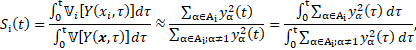
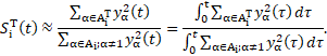
Finally, from the PCE, it is possible to estimate the two sensitivity indices as the ratio between the PCE coefficients [14]. Since the case study is dynamic, the variance of the output evolves in time. A pointwise-in-time evaluation of sensitivity indices turns out to be inaccurate in describing such evolution. Therefore, an analysis that is aware of the history of the output variability is needed. The implementation of time-dependent indices, known as generalised Sobol indices [15] reads
4. 2. Application to the thrombus formation model
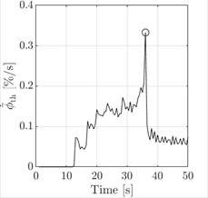
The input parameters that are considered to represent
uncertainty are listed in Table 1. To adequately cover and understand the
sensitivity of thrombus formation on the selected parameters, the volume
fraction of thrombus, the thrombus growth rate, and a characteristic growth
time ![]() are considered as the quantities of interest.
The volume fraction of thrombus expressed as a percentage is defined as
are considered as the quantities of interest.
The volume fraction of thrombus expressed as a percentage is defined as
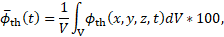
where ![]() is the domain volume and the
thrombus growth rate (
is the domain volume and the
thrombus growth rate (![]() as
as
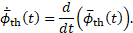
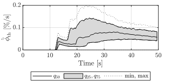
It seems promising to introduce an indicator
that describes the development of the thrombus in time. This indicator could
improve model fitting to experimental data, the introduction of a time scale in
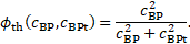
thrombus growth, or both. A characteristic growth time ![]() is therefore introduced, which is defined by
the maximum peak of the thrombus growth rate, thus the time after which the
thrombus growth rate decreases significantly. At
is therefore introduced, which is defined by
the maximum peak of the thrombus growth rate, thus the time after which the
thrombus growth rate decreases significantly. At ![]() the thrombus formation is considered almost
complete, and the thrombus is said to be developed, i.e. its volume will no
longer change significantly in time. An example of
the thrombus formation is considered almost
complete, and the thrombus is said to be developed, i.e. its volume will no
longer change significantly in time. An example of ![]() identification is illustrated in Figure 4, where
the growth rate of one typical simulation is plotted over the simulation time.
The characteristic growth time
identification is illustrated in Figure 4, where
the growth rate of one typical simulation is plotted over the simulation time.
The characteristic growth time ![]() is unique for each simulation. However, not all
simulations reached a growth rate peak in the simulation time, preventing the
assignment of the characteristic growth time. Such simulations were excluded
from the sensitivity analysis.
is unique for each simulation. However, not all
simulations reached a growth rate peak in the simulation time, preventing the
assignment of the characteristic growth time. Such simulations were excluded
from the sensitivity analysis.
The developed thrombus and its
characteristic growth time are directly connected. Acceleration or deceleration of the thrombus formation
results in a variation of ![]() in the model. For an in-depth
understanding of the growth characteristics, this relationship should be
analysed in detail.
in the model. For an in-depth
understanding of the growth characteristics, this relationship should be
analysed in detail.
Each model input factor is treated as a uniformly
distributed random variable on a given interval, since their actual values, and
distributions are not known, Table 1. The sample is produced with latin
hypercube sampling techniques with size <![]() equal to 450. The number of simulations is
bounded by the high computational cost of the model and fulfils the
requirements for the construction of the PCE. The latter is solved with the
regression LARS method through the Matlab toolbox UQlab [16], where the degree
of the polynomial is set to 3.
equal to 450. The number of simulations is
bounded by the high computational cost of the model and fulfils the
requirements for the construction of the PCE. The latter is solved with the
regression LARS method through the Matlab toolbox UQlab [16], where the degree
of the polynomial is set to 3.

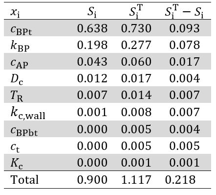
5. Results
The sensitivity indices ![]() and
and ![]() for the maximum volume fraction of thrombus are
listed in Table 2. By looking at the first column, one observes that the
first-order sensitivity indices do not sum up to one, which occurs in the
presence of non-additive model behaviour. Circa 90% of the output variance can
be attributed to
for the maximum volume fraction of thrombus are
listed in Table 2. By looking at the first column, one observes that the
first-order sensitivity indices do not sum up to one, which occurs in the
presence of non-additive model behaviour. Circa 90% of the output variance can
be attributed to ![]() ,
, ![]() , and
, and ![]() . The bounded
platelets threshold
. The bounded
platelets threshold ![]() accounts alone, i.e. without considering
interactions, for about 64% of the variation of the volume fraction of
thrombus. By subtracting the first-order from the total-order indices of Table
2, the interaction effect is estimated.
accounts alone, i.e. without considering
interactions, for about 64% of the variation of the volume fraction of
thrombus. By subtracting the first-order from the total-order indices of Table
2, the interaction effect is estimated.
Table 1. Input parameters of the thrombus model and their probabilistic distribution used for the sensitivity analysis. All input parameters follow a uniform probability distribution on the indicated interval.
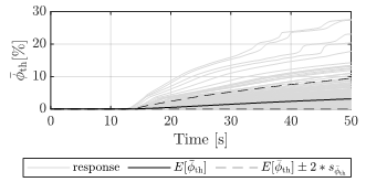
Since the thrombus develops in time, it is essential to understand how the variation of its development evolves in time. The results show several trends (Figures 5 and 6). Increasing variability in time is visible, especially towards the end of the simulation time. In Figure 5, at 50 s of simulation time, the distribution of the recorded maximum volume fraction of thrombus varies from the absence of thrombus to a thrombus coverage of circa 30% of the volume domain. Such variability is critical for a model in which the computation of the thrombus volume is an important goal.
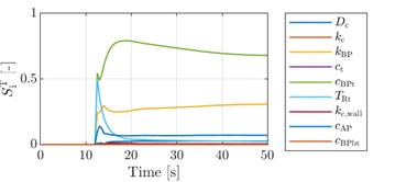
The results of the generalised total-Sobol
indices for the volume fraction of thrombus and the thrombus growth rate are
shown in Figure 7. The sensitivity analysis results do not differ for the two
quantities of interest (Eq.17 and 18); therefore, only one plot is shown.
Furthermore, the first-Sobol index does not display a trend that differs from
the total-Sobol index, suggesting a low degree of interactions between the
input random variables [17]. In Figure 7, the sensitivity analysis in time of
volume fraction of thrombus and thrombus growth rate shows the significant
influence of the bounded platelets concentration threshold ![]() . Besides this, only the bounded platelets
reaction rate
. Besides this, only the bounded platelets
reaction rate ![]() shows a comparably strong effect on the volume
fraction of thrombus.
shows a comparably strong effect on the volume
fraction of thrombus.
The other input random variables mostly have a small
or negligible effect on the output and might be considered as model constants.
The only exception is the significant role of the residence time threshold ![]() in the early stage of thrombus initiation.
in the early stage of thrombus initiation.
However, this parameter is mostly responsible
for sparking off the formation of the thrombus, while its effect on the final
thrombus size is also negligible. The influence of the coagulant diffusivity ![]() shows a small peak right after the first
formation of the thrombus, but remains low throughout the simulation time.
shows a small peak right after the first
formation of the thrombus, but remains low throughout the simulation time.
Table 2: Sobol indices of the input random variables on the maximum volume fraction of thrombosis.
As may be read from Eq. 7 and Eq. 8, bounded
platelets are generated from activated platelets in areas with low shear rate,
high residence time and high concentration of coagulant. The bounded platelets
can stop the flow if their concentration is sufficiently higher than the
threshold value, ![]() . Any variation of the bounded platelets
concentration threshold will significantly change the process of thrombus
formation, i.e. it essentially controls where and how fast the thrombus can
form. Moreover, the reaction rate
. Any variation of the bounded platelets
concentration threshold will significantly change the process of thrombus
formation, i.e. it essentially controls where and how fast the thrombus can
form. Moreover, the reaction rate ![]() determines how fast the concentration of
bounded platelets may reach the threshold value
determines how fast the concentration of
bounded platelets may reach the threshold value ![]() .
.
The interconnected roles of the two
parameters ![]() and
and ![]() on thrombus formation advocate the
idea that there might be a correlation between these parameters and a characteristic time of the thrombus formation process.
To verify if the characteristic growth time
on thrombus formation advocate the
idea that there might be a correlation between these parameters and a characteristic time of the thrombus formation process.
To verify if the characteristic growth time ![]() is the right candidate for
characterising the thrombus growth rate, a sensitivity analysis is also
performed for this quantity of interest.
is the right candidate for
characterising the thrombus growth rate, a sensitivity analysis is also
performed for this quantity of interest.
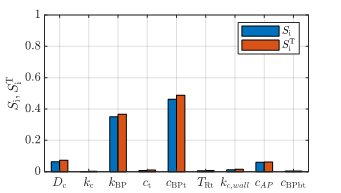
The sensitivity analysis results for the
characteristic growth time ![]() of the thrombus are shown in Figure 8. Here,
the sensitivity indices are shown in a bar plot, where the first- and
total-Sobol indices are shown side-by-side to highlight the presence of
potential interactions, given by their difference in value. The main parameters
affecting the shift in
of the thrombus are shown in Figure 8. Here,
the sensitivity indices are shown in a bar plot, where the first- and
total-Sobol indices are shown side-by-side to highlight the presence of
potential interactions, given by their difference in value. The main parameters
affecting the shift in ![]() are again the bounded platelets concentration
threshold
are again the bounded platelets concentration
threshold ![]() and the bounded platelets reaction rate
and the bounded platelets reaction rate ![]() .
.

 .
. From the results of the sensitivity analysis for ![]() (Figure 8), the characteristic growth time is a
function of
(Figure 8), the characteristic growth time is a
function of ![]() and
and ![]() . Because a high threshold
. Because a high threshold ![]() delays thrombus growth, while a high reaction
rate
delays thrombus growth, while a high reaction
rate ![]() has an accelerating effect, the ratio between them
is introduced as a characteristic growth rate
has an accelerating effect, the ratio between them
is introduced as a characteristic growth rate ![]() of the model,
of the model,

with the dimension of a
cubic meter per second (![]() ). Its relationship to the characteristic growth
time
). Its relationship to the characteristic growth
time ![]() is shown in Figure 9. Here, the data are
produced with the computation of the metamodel for the characteristic growth
time considering all input parameters, except for <
is shown in Figure 9. Here, the data are
produced with the computation of the metamodel for the characteristic growth
time considering all input parameters, except for <![]() and
and ![]() , as constants. The data was fit with non-linear
regression. A low value of the characteristic growth rate
, as constants. The data was fit with non-linear
regression. A low value of the characteristic growth rate ![]() leads to high values of
leads to high values of ![]() , that can be interpreted as a delayed thrombus
growth. Such behaviour is a consequence of a low value of bounded platelets
reaction rate
, that can be interpreted as a delayed thrombus
growth. Such behaviour is a consequence of a low value of bounded platelets
reaction rate ![]() , and a high bounded platelets concentration
threshold
, and a high bounded platelets concentration
threshold ![]() . In the case of high
. In the case of high ![]() , the required number of bounded platelets to
form a thrombus has to be higher, and therefore its growth is reduced.
, the required number of bounded platelets to
form a thrombus has to be higher, and therefore its growth is reduced.
The data have been fitted by
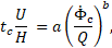
where ![]() is the model convection time given
by the ratio of inlet velocity magnitude
is the model convection time given
by the ratio of inlet velocity magnitude ![]() and
inlet height
and
inlet height ![]() ,
, ![]() is the volumetric flow rate, where
the area
is the volumetric flow rate, where
the area ![]() is
the product of inlet height
is
the product of inlet height ![]() and geometry depth
and geometry depth ![]() m.
The constants
m.
The constants ![]() and
and
![]() are
computed by non-linear regression analysis. Their values, together with their
95% confidence intervals, are:
are
computed by non-linear regression analysis. Their values, together with their
95% confidence intervals, are: ![]() , and
, and ![]() . The coefficient of determination
. The coefficient of determination ![]() .
.
Such a formulation of the characteristic growth time of the thrombus appears as a promising tool for the modelling phase. By varying the characteristic growth rate of the problem, it is possible to accelerate or inhibit the thrombus formation.
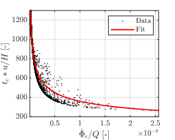 normalised by convection time
  as a function of the characteristic
growth rate
as a function of the characteristic
growth rate  normalised by volumetric flow rate
6. Conclusions
The thrombus formation model presents a high amount of variation due to the intrinsic uncertainty of the input parameters, which are usually collected from different literature sources. The input variation is modelled with uniform probability distributions for nine model input random variables, and a sensitivity analysis is performed through the construction of a polynomial chaos expansion metamodel. To better grasp the model variation for the scope of the study, the quantities of interest are considered to be the volume fraction of thrombus, the thrombus growth rate, and the time instant at which the growth rate peak is recorded, namely the characteristic growth time.
Input parameters such as the bounded
platelets reaction rate ![]() and the bounded platelets concentration
threshold of activated platelets
and the bounded platelets concentration
threshold of activated platelets ![]() , show high sensitivity indices, and
therefore their proper determination requires further investigation. In
general, the input parameters that include the platelet's mechanics control
most of the process, except for the bounded platelets threshold at the boundary
, show high sensitivity indices, and
therefore their proper determination requires further investigation. In
general, the input parameters that include the platelet's mechanics control
most of the process, except for the bounded platelets threshold at the boundary
![]() . All the other input random
variables, including the parameters relating to the coagulant, have little to
no influence on the considered outputs, and therefore they could be switched to
fixed values without altering the model response.
. All the other input random
variables, including the parameters relating to the coagulant, have little to
no influence on the considered outputs, and therefore they could be switched to
fixed values without altering the model response.
The results of the sensitivity
analysis for the model outputs show that the bounded platelets threshold ![]() exerts the most substantial
influence. The reaction rate of bounded platelets
exerts the most substantial
influence. The reaction rate of bounded platelets ![]() plays the second-largest role in
the thrombus growth rate and the volume fraction of thrombus.
plays the second-largest role in
the thrombus growth rate and the volume fraction of thrombus.
Finally, the introduced characteristic
growth rate ![]() appears to be a promising indicator
for the speed of thrombus formation. This characteristic rate is supposed to be
beneficial for fitting model results to experimental results, in-turn improving
the haemodynamic-based model in predicting thrombus formation on a proper time
scale.
appears to be a promising indicator
for the speed of thrombus formation. This characteristic rate is supposed to be
beneficial for fitting model results to experimental results, in-turn improving
the haemodynamic-based model in predicting thrombus formation on a proper time
scale.
Acknowledgement
This work is supported by the Graz University of Technology through the LEAD Project "Mechanics, Modeling, and Simulation of Aortic Dissection".
References
[1] C.A. Nienaber, R.E. Clough, N. Sakalihasan, T. Suzuki, R. Gibbs, F. Mussa, M.P. Jenkins, M.M. Thompson, A. Evangelista, J.S.M. Yeh, N. Cheshire, U. Rosendahl & J. Pepper "Aortic dissection". In: Nature Reviews Disease Primers 2.1 (2016), pp. 1-18. View Article
[2] C. Menichini and X.Y. Xu. "Mathematical modeling of thrombus formation in idealised models of aortic dissection: initial findings and potential applications". In: Journal of mathematical biology 73.5 (2016), pp. 1205-1226. View Article
[3] T.T. Tsai, A. Evangelista, C.A. Nienaber, T. Myrmel, G. Meinhardt, J.V. Cooper, D.E. Smith, T. Suzuki, R. Fattori, A. Llovet, J. Froehlich, S. Hutchison, A. Distante, T. Sundt, J. Beckman, J.L. Januzzi, E.M. Isselbacher, K.A. Eagle. "Partial thrombosis of the false lumen in patients with acute type B aortic dissection". In: New England Journal of Medicine 357.4 (2007), pp. 349-359. View Article
[4] Y. Bernard, H. Zimmermann, S. Chocron, J-F. Litzler, B. Kastler, J-P. Etievent, N. Meneveau, F. Schiele, J-P. Bassand. "False lumen patency as a predictor of late outcome in aortic dissection". In: The American journal of cardiology 87.12 (2001), pp. 1378-1382. View Article
[5] S. Trimarchi, J.L. Tolenaar, F.H.W. Jonker, B. Murray, T.T. Tsai, K.A.Eagle, V. Rampoldi, H.J.M. Verhagen, J.A.van Herwaarden, F.L. Moll, B.E. Muhs, J.A. Elefteriades Importance of false lumen thrombosis in type B aortic dissection prognosis. 2013. View Article
[6] C. Menichini, Z.Cheng, R.G.J. Gibbs and X.Y. Xu "Predicting false lumen thrombosis in patients-specific models of aortic dissection". In: Journal of The Royal Society Interface 13.124 (2016), p. 20160759. View Article
[7] B. Sudret. "Global sensitivity analysis using polynomial chaos expansions". In: Reliability engineering & system safety 93.7 (2008), pp. 964-979. View Article
[8] J.O. Taylor, K.P. Witmer, T. Neuberger, B.A. Craven, R.S. Meyer, S. Deutsch, K.B. Manning "In vitro quantification of time dependent thrombus size using magnetic resonance imaging and computational simulations of thrombus surface shear stresses". In: Journal of biomechanical engineering 136.7 (2014). View Article
[9] J.O. Taylor, R.S. Meyer, S. Deutsch, K.B. Manning "Development of a computational model for macroscopic predictions of device-induced thrombosis". In: Biomechanics and modeling in mechanobiology 15.6 (2016), pp. 1713-1731. View Article
[10] G. Biswas, M. Breuer, F. Durst. "Backward-facing step flows for various expansion ratios at low and moderate Reynolds numbers." J. Fluids Eng. 126, no. 3 (2004): 362-374. View Article
[11] I. M. Sobol. "Global sensitivity indices for nonlinear mathematical models and their Monte Carlo estimates". In: Mathematics and computers in simulation 55.1-3 (2001), pp. 271-280. View Article
[12] R. G. Ghanem, P. D. Spanos. Stochastic Finite elements: a spectral approach. Courier Corporation, 2003.
[13] D. Xiu and G. E. Karniadakis. "The Wiener-Askey polynomial chaos for stochastic differential equations". In: SIAM journal on scientific computing 24.2 (2002), pp. 619-644. View Article
[14] T. Crestaux, O. Le Maître, and J. Martinez. "Polynomial chaos expansion for sensitivity analysis". In: Reliability Engineering & System Safety 94.7 (2009), pp. 1161-1172. View Article
[15] A. Alexanderian, P. A. Gremaud, and R. C. Smith. "Variance-based sensitivity analysis for time-dependent processes". In: Reliability Engineering & System Safety, 196 (2020), pp. 106722. View Article
[16] S. Marelli and B. Sudret. "UQLab: A framework for uncertainty quantification in Matlab". In: Vulnerability, uncertainty, and risk: quantification, mitigation, and management. 2014, pp. 2554-2563. View Article
[17] Melito, G. M., Jafarinia, A., Hochrainer, T., & Ellermann, K. (2020, July). "Sensitivity analysis of a hemodynamic-based model for thrombus formation and growth". In: Proceedings of the 6th World Congress on Electrical Engineering and Computer Systems and Sciences (EECSS'20): ICBES'20 (2020), pp. ICBES-127.View Article