Journal of Biomedical Engineering and Biosciences (JBEB)
ISSN: 2564-4998

Volume 7 - Year 2020 - Pages 13-24
DOI: 10.11159/jbeb.2020.002
Blood Rheology Influence on False Lumen Thrombosis in Type B Aortic Dissection
Alireza Jafarinia1*, Thomas Stephan Müller2, Ursula Windberger3, Günter Brenn2, Thomas Hochrainer1
1Institute of Strength of Materials/Graz University of Technology
Kopernikusgasse 24/I, Graz, Austria
alireza.jafarinia@tugraz.at; hochrainer@tugraz.at
2Institute of Fluid Mechanics and Heat Transfer/Graz University of Technology
Inffeldgasse 25/F, Graz, Austria
t.mueller@tugraz.at; guenter.brenn@tugraz.at
3Center of Biomedical Research/Medical University of Vienna
Währingergürtel 18-20, 1090 Vienna, Austria
ursula.windberger@meduniwien.ac.at
Abstract - Aortic dissection is a disease caused by the occurrence of a rupture in the innermost layer of the aortic wall. Due to the pulsation of the heart, blood penetrates through the tear between the layers of the aortic wall, which causes a new, so-called false lumen (FL). The local haemodynamic conditions in the FL significantly contribute to clotting of blood, so the formation of a thrombus. The level of thrombosis in the FL affects patients’ prognosis and chances of survival, in which a complete thrombosis is usually beneficial. In recent studies on platelet deposition in the FL, it is demonstrated that haemodynamic conditions influence on platelet activation and aggregation, effectively boosting in regions of recirculation. Blood coagulation has the highest chance of occurrence in these recirculation regions within the FL. Considering the dominant influence of shear rate in FL thrombosis, the non-Newtonian rheological properties and behaviour of blood play a crucial role. The most important rheological factor is the volume fraction of red blood cells in the blood, i.e., the haematocrit value (HCT), which affects the shear rate dependent viscosity and the yield stress observed in regions of low shear rate and stress, respectively, in the blood flow. In the current work, the influence of the haematocrit value on thrombosis in the FL is simulated. The simulations are done in idealized aortic dissection phantom models employing HCT-dependent non-Newtonian haemodynamics. The value for the HCT was varied within a physiological range. On the one hand, an increase in the total volume of thrombus in time was found for all HCT values. On the other hand, with increasing HCT values, less thrombus is formed in the FL. This suggests that high HCT values impede thrombus formation due to rheological effects and that patients with higher haematocrit values have less chance of benefiting from complete thrombosis in the FL.
Keywords: Aortic Dissection, Thrombus Formation, Haematocrit, Shear-Thinning Fluid, Carreau Model.
© Copyright 2020 Authors This is an Open Access article published under the Creative Commons Attribution License terms. Unrestricted use, distribution, and reproduction in any medium are permitted, provided the original work is properly cited.
Date Received: 2020-10-16
Date Accepted: 2020-11-03
Date Published: 2020-11-30
1. Introduction
The disease is initiated by the perforation of the inner layer of the aortic wall, causing its layers to delaminate. As the delamination progresses, a new volume, the so-called FL, is created; hence, the blood flow bifurcates partially from the main blood flow, in the descending part of the aorta (true lumen, TL), into the FL. The tear causes the FL propagation due to the pulsation of the blood flow and eventually, a second tear (re-entry tear) may occur in the descending part of the aorta, merging the flows of both lumens.
The haemodynamic conditions in the FL, including flow disturbance, recirculation, and considerable variability in wall shear stress (WSS), might contribute to the formation and growth of a thrombus [2]. There exist three cases of FL thrombosis in TBAD, i.e., patent, partial, and complete thrombosis. Tsai et al. [3] showed that partial thrombosis is associated with a high mortality rate, whereas complete thrombosis of the FL improves patients’ prognosis [4,5]. Therefore, it is important to investigate and understand under which conditions complete thrombosis of the FL occurs.
Thrombus formation is a complex phenomenon comprising many biological and chemical processes. Until now, it is unclear why thrombosis does or does not occur during the course of aortic dissection. Thrombosis, in the case of aortic dissection, is dominated by haemodynamic conditions, and it is enhanced in low shear rate regions in the FL [5]. In recent studies on platelet deposition it is demonstrated that the change in haemodynamic conditions in the FL effectively boosts platelet activation and aggregation in regions of recirculation [6]. Blood coagulation has the highest chance of occurrence in these recirculation regions within the FL, where the shear rates are significantly lower than in the TL [7]. Considering the dominant influence of shear rate in FL thrombosis, the rheological behaviour of blood plays a crucial role. Blood is a suspension with a non-Newtonian rheological behaviour exhibiting shear thinning and yield stress. Blood rheology mainly depends on the volume fraction of red blood cells, i.e., the haematocrit value [8], which varies from person to person, ranging between 30 and 55 percent. In the current work, we study the influence of the haematocrit value on thrombosis in the FL.
For the thrombus formation simulation, the haemodynamic-based mathematical model in the present study developed by Menichini et al. ([2,9]) is used. In this model, the formation process is primarily controlled by haemodynamics, which are determined by the rheological properties of blood, making it suitable for investigating the influence of HCT variation.
To describe the shear-dependent behaviour of blood, the Carreau model is used [10]. The four parameters of the model are obtained by blood rheometry. The rheological model incorporates an additional rheological phenomenon of blood, the tendency of red blood cells to agglomerate and form so-called rouleaux. Those rouleaux need a minimum of shear stress to be broken up; thus, a yield stress is accounted for in the model. In our previous study [11], we investigated the influence of six different HCT values on false lumen thrombosis. Because the results showed low sensitivity on the HCT value in the intermediate range, we will focus only on three HCT values; low (35 %), average (45 %), and high (55 %). All the numerical simulations are carried out in the open source software OpenFOAM.
The paper is organised as follows: the next section presents the model of thrombus formation; section 3 gives the rheological modelling and section 4 presents the problem formulation. In Section 5 the computational fluid dynamics are given, followed by the results and the conclusions.
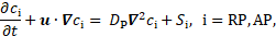
2. Governing Equations
2.1. Fluid dynamics
The blood is modelled as an incompressible fluid
with constant density ![]() , such that the balance of mass reduces to the
solenoidality of the velocity field
, such that the balance of mass reduces to the
solenoidality of the velocity field ![]() , i.e.,
, i.e.,

The flow in the aortic arch and FL is modelled by a modified form of the Navier-Stokes equations
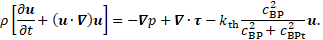
with pressure ![]() and the
extra stress tensor
and the
extra stress tensor ![]() , which will
be introduced in Section 3. The thrombus model, which will be detailed in the
next subsection, distinguishes three types of platelets, i.e., resting,
activated, and bounded platelets. A high concentration of bounded platelets
, which will
be introduced in Section 3. The thrombus model, which will be detailed in the
next subsection, distinguishes three types of platelets, i.e., resting,
activated, and bounded platelets. A high concentration of bounded platelets ![]() indicates the presence of a thrombus. To
account for the thrombus in the flow field, the right-hand `sink term’ in Eq. 2
is introduced, which obstructs the flow in high
indicates the presence of a thrombus. To
account for the thrombus in the flow field, the right-hand `sink term’ in Eq. 2
is introduced, which obstructs the flow in high ![]() areas. The quantity
areas. The quantity
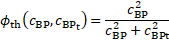
is interpreted as degree
of local thrombosis. This function takes values between ![]() and
and ![]() , in
dependence of the bounded platelet concentration relative to the threshold
value
, in
dependence of the bounded platelet concentration relative to the threshold
value ![]() , (Table 1). The value of the coefficient
, (Table 1). The value of the coefficient ![]() (Table 2) in the sink term is chosen large
enough to stop the flow where the thrombus is formed [2].
(Table 2) in the sink term is chosen large
enough to stop the flow where the thrombus is formed [2].
2.2. Thrombus Formation
The model of Menichini et al. [2] controls the
formation of the thrombus based on wall shear stress, shear rate![]() , a so-called
residence time
, a so-called
residence time ![]() , as well as the concentrations of coagulant
, as well as the concentrations of coagulant ![]() , resting platelets
, resting platelets
![]() , activated platelets
, activated platelets ![]() and, ultimately, bounded platelets
and, ultimately, bounded platelets ![]() . The model achieves reasonable simulation times
for thrombus growth by modelling the reaction equations partly based on
so-called cycle-averaged field variables, which are indicated by overbars. The
cycle average of a field variable
. The model achieves reasonable simulation times
for thrombus growth by modelling the reaction equations partly based on
so-called cycle-averaged field variables, which are indicated by overbars. The
cycle average of a field variable ![]() is defined as
is defined as
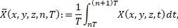
where ![]() denotes the
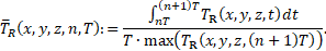
length of a cardiac cycle, while n is the cycle counter starting from 0. An
exception to this rule is the definition of the cycle-averaged residence time
denotes the
length of a cardiac cycle, while n is the cycle counter starting from 0. An
exception to this rule is the definition of the cycle-averaged residence time ![]() , which is additionally normalized by the maximum
value of
, which is additionally normalized by the maximum
value of ![]() in the field, at the end of the corresponding
cycle,
in the field, at the end of the corresponding
cycle,
Thrombus growth is limited or enhanced depending
on threshold values for cycle-averaged wall shear stress, shear rate, residence
time, as well as concentrations of bounded platelets and coagulant. The
threshold values are indicated by an additional subscript ![]() .
.
The central quantity for thrombus growth in the
model is the concentration of bounded platelets ![]() , which appears in Eq. 2. Regions with high
concentrations of bounded platelets are considered as thrombus, where the blood
flow gets inhibited by the modification of the momentum balance, Eq. 2. Bounded
platelets are generated from activated platelets
, which appears in Eq. 2. Regions with high
concentrations of bounded platelets are considered as thrombus, where the blood
flow gets inhibited by the modification of the momentum balance, Eq. 2. Bounded
platelets are generated from activated platelets ![]() through the reaction equation
through the reaction equation
where the reaction rate is determined by a reaction
constant ![]() (Table 2), the coagulant concentration
(Table 2), the coagulant concentration ![]() , and cycle-averaged
shear rate
, and cycle-averaged
shear rate ![]() and
residence time
and
residence time ![]() ; each time in dependence on their according
threshold values which are available in Table 1. Activated platelets are
generated by `activating’ resting platelets. To avoid numerical ill
conditioning,
; each time in dependence on their according
threshold values which are available in Table 1. Activated platelets are
generated by `activating’ resting platelets. To avoid numerical ill
conditioning, ![]() and
and ![]() are considered as the normalized number density
of the according species in the blood by [2],
are considered as the normalized number density
of the according species in the blood by [2],
 and
and 
with the initial number
densities ![]() and
and ![]() . The transport equations for resting and
activated platelets are convection-diffusion-reaction equations of the form
. The transport equations for resting and
activated platelets are convection-diffusion-reaction equations of the form
where

with ![]() and
and ![]() being reaction constants (Table 2). Red blood
cells have a shear-dependent effect on the transport of platelets. One way to
simulate it is by adjusting Brownian diffusion fluxes.
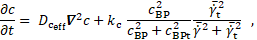
being reaction constants (Table 2). Red blood
cells have a shear-dependent effect on the transport of platelets. One way to
simulate it is by adjusting Brownian diffusion fluxes. ![]() denotes the diffusion coefficient of platelets,
which is enhanced due to shear rate through the following equation [2]
denotes the diffusion coefficient of platelets,
which is enhanced due to shear rate through the following equation [2]
with the Brownian diffusivity
![]() and the coefficient
and the coefficient ![]() [2].
[2].
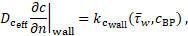
The coagulant concentration ![]() represents
the lumped effect of all underlying biochemical reactions in the coagulation
cascade [2]. In low
shear rate areas, there is a production of coagulant at the wall based on the
conditions specified at the boundary. The diffusion-reaction equation for the
coagulant concentration is
represents
the lumped effect of all underlying biochemical reactions in the coagulation
cascade [2]. In low
shear rate areas, there is a production of coagulant at the wall based on the
conditions specified at the boundary. The diffusion-reaction equation for the
coagulant concentration is
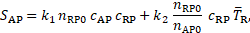
in which ![]() is a reaction constant (Table 2) and
is a reaction constant (Table 2) and ![]() an effective diffusion coefficient of the form
an effective diffusion coefficient of the form
with ![]() , which gets enhanced in areas of low cycle-averaged
shear rates [2].
, which gets enhanced in areas of low cycle-averaged
shear rates [2].
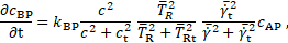
The reactive source term
in Eq. 12 shows that the coagulant is produced where bounded platelets
concentration is sufficiently higher than its threshold value (![]() ) and the cycle-averaged shear rate is lower
than its threshold value (
) and the cycle-averaged shear rate is lower
than its threshold value (![]() ). The decisive production of coagulant
concentration (which is assumed to be identically zero, initially), however,
happens at the vessel wall via a Neumann boundary condition. The coagulant flux
into the domain through the wall is given by
). The decisive production of coagulant
concentration (which is assumed to be identically zero, initially), however,
happens at the vessel wall via a Neumann boundary condition. The coagulant flux
into the domain through the wall is given by
where ![]() is a reaction constant. If the cycle-averaged
wall shear stress
is a reaction constant. If the cycle-averaged
wall shear stress ![]() is larger than the threshold value 0.2 Pa and the
concentration of bounded platelets at the wall is larger
is larger than the threshold value 0.2 Pa and the
concentration of bounded platelets at the wall is larger ![]() then
then![]() is zero, while otherwise
is zero, while otherwise ![]()
The so-called residence time ![]() of liquid components or platelets in the field,
is determined by the transport equation
of liquid components or platelets in the field,
is determined by the transport equation
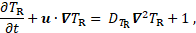
where ![]() is the self-diffusivity of blood. High
residence time marks areas where the platelets spend long time [2].
is the self-diffusivity of blood. High
residence time marks areas where the platelets spend long time [2].
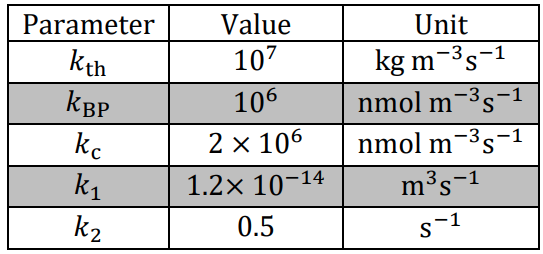
Table 1: Threshold values in the thrombus formation model.
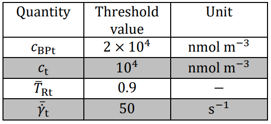
Table 2: Reaction constants in the thrombus formation model.
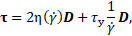
3. Rheological Modelling
The rheological model of blood as a shear-thinning liquid with a yield stress determines the extra stress as a function of the rate-of-deformation tensor
 if
if 
 if
if 
with the rate-of-deformation
tensor ![]() (in Cartesian coordinates x, y for i or j = 1,
2) defined as
(in Cartesian coordinates x, y for i or j = 1,
2) defined as
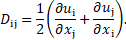
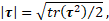
Therefore, the fluid
does not flow if the stress magnitude is below the yield stress. Whereas the
arguments ![]() and
and ![]() originate
from the invariants of extra stress tensor
originate
from the invariants of extra stress tensor ![]()
and the
rate-of-deformation tensor ![]()

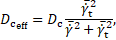
In these equations, the shear-rate dependent viscosity and the yield stress appear as liquid material properties, which are modelled as laid out in the following two sub-sections.
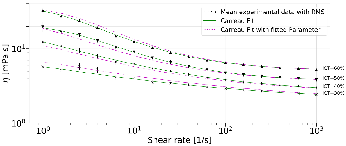
3.1. Shear-Rate Dependent Viscosity
Shear rheometric data of human blood was
measured by a rheometer with a double cylindrical gap geometry for shear rates
ranging from ![]() to
to ![]() . The flow curves were obtained for four
different haematocrit values (HCT=30%-60%, with a gradation of 10%) from five
different test persons. The shear-thinning, inelastic behaviour of blood
qualifies the Carreau model
. The flow curves were obtained for four
different haematocrit values (HCT=30%-60%, with a gradation of 10%) from five
different test persons. The shear-thinning, inelastic behaviour of blood
qualifies the Carreau model

for representing the
flow curves. The four quantities ![]() ,
, ![]() ,
, ![]() and
and ![]() are free
model parameters to be determined in fitting the model equation to measurement
data. The data are shown in Figure 1. The green curves represent the fits with
the Carreau model. For evaluating the viscosity at HCT values intermediate to
the experiments, a fit of the model parameters was performed. Thus, all four
parameters were available as functions of the HCT value. The pink curves
correspond to the viscosities calculated with the parameters from the fit for
the corresponding haematocrit, as noted next to the curves.
are free
model parameters to be determined in fitting the model equation to measurement
data. The data are shown in Figure 1. The green curves represent the fits with
the Carreau model. For evaluating the viscosity at HCT values intermediate to
the experiments, a fit of the model parameters was performed. Thus, all four
parameters were available as functions of the HCT value. The pink curves
correspond to the viscosities calculated with the parameters from the fit for
the corresponding haematocrit, as noted next to the curves.
3.2. Yield Stress
The incorporation of a
yield stress in the rheological model is based on the mathematical formulation
by Merrill [12] as a piece-wise function of the haematocrit value HCT. The
model equation for 30% ![]() HCT
HCT ![]() 50% is
50% is

and for HCT > 50% is
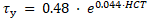
The equations reveal the yield stress in milli-Pascal with the HCT inserted in percent. The model approximation to the experimental data available in the literature is shown in Figure 2.
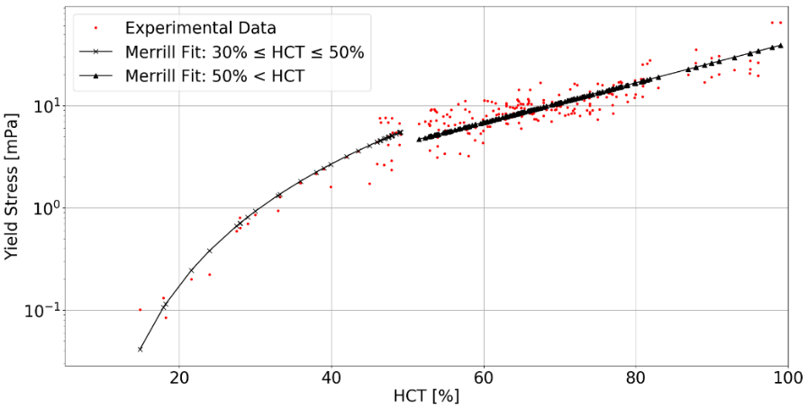
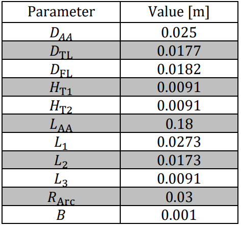
4. Problem Formulation
Thrombus formation in the case of TBAD was
investigated on the 2D geometry of an abstracted aorta given in Figure 3, with
the geometrical parameters in Table 3. For the sake of simplicity, only the
ascending aorta, aortic arch without carotid arteries, and the descending part
of the thoracic aorta were considered. The dissection is realized by splitting
up the descending part of the aorta into a TL and a FL with the width ![]() and
and ![]() , respectively. Both lumens are connected via a
proximal and a distal tear. The proximal tear is located at the reference line
, respectively. Both lumens are connected via a
proximal and a distal tear. The proximal tear is located at the reference line ![]() and the distal one at
and the distal one at ![]() . Their width is
. Their width is ![]() and
and ![]() , respectively. The ascending part of the aorta
has the width
, respectively. The ascending part of the aorta
has the width ![]() and length
and length ![]() . The width of the aortic arch is equal to the
one of the ascending part. The radius of curvature is described by
. The width of the aortic arch is equal to the
one of the ascending part. The radius of curvature is described by ![]() . The arch ends at the angle α. B is the
width of the aortic wall.
. The arch ends at the angle α. B is the
width of the aortic wall.
Table 3: Parameters of the geometry. ![]() = 45°
= 45°
5. Computational Fluid Dynamics
The model equations were solved with the finite volume method using the open-source software OpenFOAM. The 2D geometry of the flow domain was discretized into 16000 hexahedral cells, with a refining grading towards the walls to correctly resolve the gradients on the wall surface. A grid independency study was performed to ensure that a refinement of the spatial discretization would not change the outcome of the value for the volume fraction of thrombus in the FL. For the numerical schemes, a second-order implicit scheme for the time was chosen, gradient schemes with a second-order central difference and divergence schemes were calculated with a Gaussian first or second-order scheme. The non-orthogonality of wall-normal gradients was taken into account by using an appropriate correction scheme. Laplacian terms are calculated linearly limited by a value of unity. For each simulation, first the periodic solution is reached, and then the thrombus formation equations are included. For the inlet boundary condition of the velocity, a parabolic profile taken from [13] was imposed, with the no-slip condition for walls. Further details about the boundary conditions for the thrombus formation equations may be found in [2] and [9].
The heart rate simulated is 60bpm and, therefore, each cardiac cycle is nominally one second. Note though that the time-scale of thrombus formation in the employed model may not be taken by face value [2], and the times discussed in the sequel are not actual time predictions for thrombus growth.
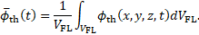
6. Results
The formation of a thrombus is indicated by the
parameter ![]() as introduced in section 2. Complete thrombosis
for a cell is reached, if
as introduced in section 2. Complete thrombosis
for a cell is reached, if ![]() approaches the value 1. Though the value of
unity may not be reached, this parameter shows a clear bimodal distribution of
values, which are effectively either zero or larger than 0.98. Note though,
that the concentration of bounded platelets affects the flow whenever
approaches the value 1. Though the value of
unity may not be reached, this parameter shows a clear bimodal distribution of
values, which are effectively either zero or larger than 0.98. Note though,
that the concentration of bounded platelets affects the flow whenever ![]() . A measure of the volume fraction of thrombus
is defined through the following formula (normalized different from [11]), to
quantify the fraction of thrombus in the false lumen,
. A measure of the volume fraction of thrombus
is defined through the following formula (normalized different from [11]), to
quantify the fraction of thrombus in the false lumen,
The rate of thrombosis, subsequently also referred to as thrombus growth rate is
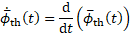
In order to decrease the necessary computation time, the model for thrombus formation is artificially accelerated by making thrombus growth depending on cycle averaged quantities. This results in two different time scales, a haemodynamical one and one for the thrombus growth, neither of which represents the physical time scale. The times provided in the following should only be viewed as a relative quantity between the different simulations.
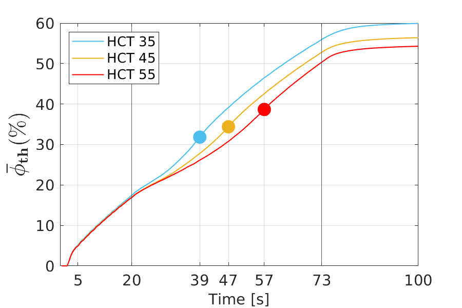
Figure 4 shows the volume fraction of thrombus in the FL as a function of time. The simulations were performed for three different haematocrit values: HCT = 35% (turquoise), 45% (yellow) and 55% (red). All simulations were run for 200 cardiac cycles to ensure the stagnation of growth for all cases. However, in all cases this stagnation was reached after 100 cycles at the latest.
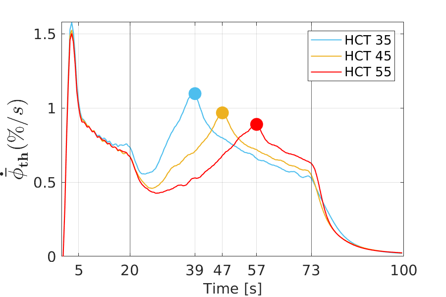
For all HCT values, the same general trend can be seen in time, with an increase in the amount of formed thrombus. Furthermore, by increasing the HCT values, less thrombus is formed in the FL. In the early stages of thrombus formation up to approximately 20 cardiac cycles, the difference in relative thrombosis for different HCT values is marginal. As time progresses, the difference of the values becomes pronounced. In all three cases, after 73 cardiac cycles, thrombus formation slows down and reaches an asymptotic value, i.e., thrombus formation effectively stops. The final values for the volume fraction of thrombus, which are anti-proportional to the haematocrit value, are 60%, 57% and 54%. The markers in Figure 4 indicate the points with the maximum growth rate. Thus, it represents a turning point in the growth behaviour, from which on the growth rate steadily slows down. The thrombus growth rate over time for the different cases is provided in Figure 5.
From a qualitative point of view, the growth rates all behave in the same way: an early sharp maximum at the very beginning, followed by a steep decrease in growth and dropping into a valley (local minimum), which is followed by a region of constantly increasing growth rate. After it has reached another peak (local maximum), the growth decreases and is constantly decreasing over a long period of the simulation time, until another characteristic point is reached. At this point, the rate of growth diminishes abruptly and subsequently tends towards zero.
An also quantitatively almost identical behaviour applies to all three cases up to about 20 cardiac cycles. The main differences occur between 20 and 73 cardiac cycles. The higher the haematocrit value, the later the local minimum and second local maximum occur. Thus, a higher haematocrit causes a delay in the characteristic points in the growth behaviour. These points are shown in Figure 5; the values are 39s, 47s and 57s, respectively.
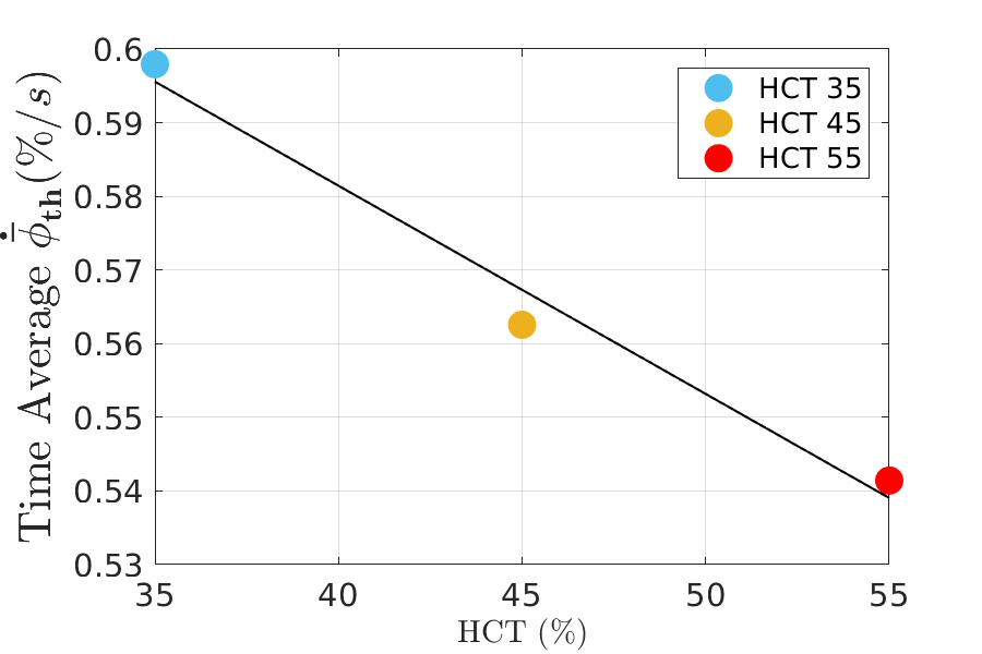
Qualitatively, the behaviour of the growth rate parallels the one of the volume fraction of thrombus: the lower the haematocrit, the higher the growth rate. This trend is displayed in form of the time averaged growth rate in Figure 6.
7. Discussion
Due
to the fact that the growth behaviour of all cases behaves qualitatively in the
same way, the case for 35% haematocrit shall serve as representative for all
cases for the purpose of discussing and explaining the interactions of thrombus
growth and haemodynamics. Figure 7 depicts snapshots of the progression of
thrombosis by means of the volume fraction of thrombus (colour coding refers to
the quantity ![]() ) at different characteristic points in time
during the simulation. The early stage of thrombus formation is shown after 5
cardiac cycles (Figure 7a). Initially, the thrombus is forming within the wake
areas above the proximal and below the distal tear. These regions exhibit low
shear rates and high residence time and are predestined for thrombosis. The
next characteristic behaviour occurs after 20 cardiac cycles (Figure 7b), as
soon as those two wake areas are fully covered with thrombus; the growth rate
drops to its intermediate minimum (see Figure 5). From this point on, the
difference in the rheological properties becomes apparent. After 25 cycles
(Figure 7c), the two thrombi in the wake areas start growing further into the
FL. The time span between the valley (local minimum) and the following peak
(local maximum) can be attributed to the growth of the two thrombus fronts from
top and bottom. The growth rate reaches its maximum at the point when the two
fronts merge (Figure 7d). For the given geometry, there is no further growth in
previously uncovered areas. Hence, until 73 cycles (Figure 7e) the growth
continuous only in the FL at the surface of the existing thrombus. The last
characteristic point, at which growth begins to stagnate, indicates a kind of
stationary state at which the haemodynamical condition at the wall and thrombus
front prevent further grow (Figure 7f).
) at different characteristic points in time
during the simulation. The early stage of thrombus formation is shown after 5
cardiac cycles (Figure 7a). Initially, the thrombus is forming within the wake
areas above the proximal and below the distal tear. These regions exhibit low
shear rates and high residence time and are predestined for thrombosis. The
next characteristic behaviour occurs after 20 cardiac cycles (Figure 7b), as
soon as those two wake areas are fully covered with thrombus; the growth rate
drops to its intermediate minimum (see Figure 5). From this point on, the
difference in the rheological properties becomes apparent. After 25 cycles
(Figure 7c), the two thrombi in the wake areas start growing further into the
FL. The time span between the valley (local minimum) and the following peak
(local maximum) can be attributed to the growth of the two thrombus fronts from
top and bottom. The growth rate reaches its maximum at the point when the two
fronts merge (Figure 7d). For the given geometry, there is no further growth in
previously uncovered areas. Hence, until 73 cycles (Figure 7e) the growth
continuous only in the FL at the surface of the existing thrombus. The last
characteristic point, at which growth begins to stagnate, indicates a kind of
stationary state at which the haemodynamical condition at the wall and thrombus
front prevent further grow (Figure 7f).
In order to understand the growth characteristics, the cycle-averaged shear rate, which primarily controls thrombus growth in the employed model, is discussed.
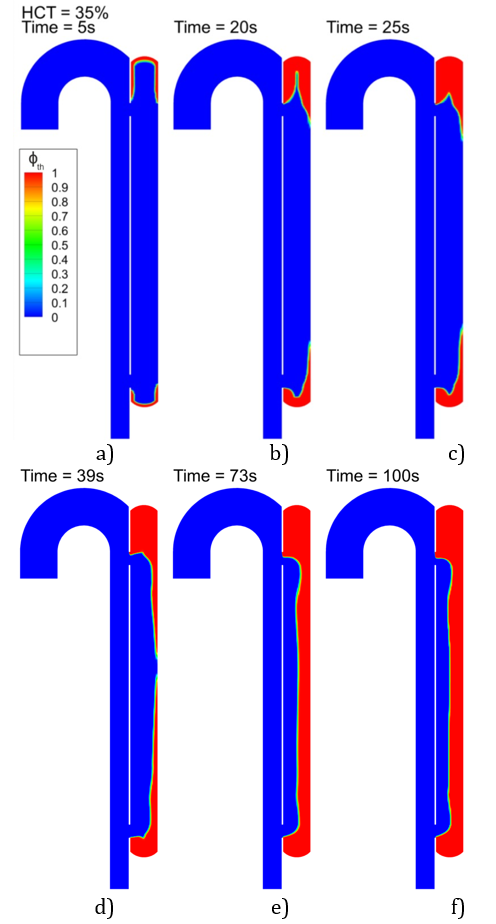
 . a) Thrombus initiation. b) After 20 cycles:
differences appear between different HCTs. c) After 25 cycles: initiation of
the growth rate increase. d) After 39 cycles: local maximum. e) After 73
cycles: a steep decline in growth rate. f) After 100 cycles: approaching to zero
growth rate.
. a) Thrombus initiation. b) After 20 cycles:
differences appear between different HCTs. c) After 25 cycles: initiation of
the growth rate increase. d) After 39 cycles: local maximum. e) After 73
cycles: a steep decline in growth rate. f) After 100 cycles: approaching to zero
growth rate. In Figure 8, the
cycle-averaged shear rate is depicted for HCT 35% at the same six different
simulation times, as previously discussed. The threshold value of the cycle-
averaged shear rate is ![]() , above which the production of coagulant and
bounded platelets ceases, compare Eqs. (12) and (6), respectively.
, above which the production of coagulant and
bounded platelets ceases, compare Eqs. (12) and (6), respectively.
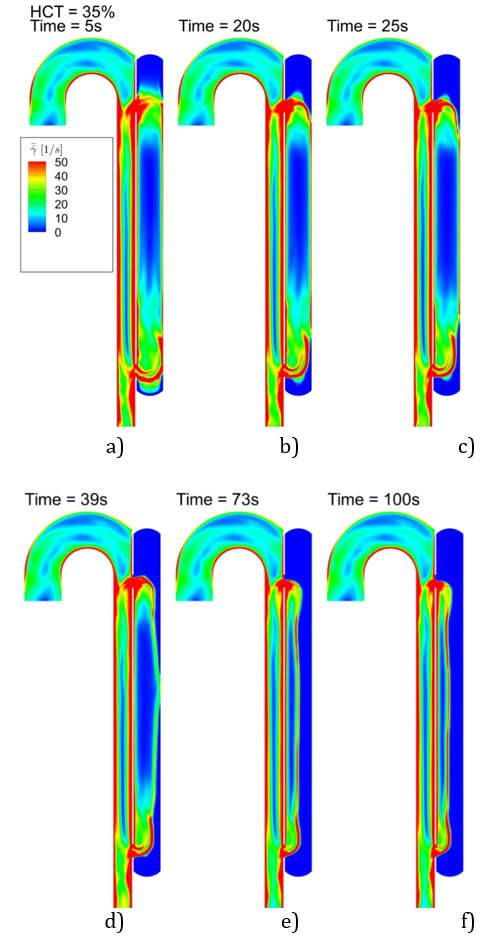
An according maximum value is chosen for the colour coding in Figure 8, to facilitate identifying the areas in which this threshold value is exceeded. No thrombus formation is observed where the cycle-averaged shear rate exceeds he threshold value.
The shear rates displayed in Figure 8 explain the observed growth behaviour: due to the low average shear rates, thrombus formation starts in the wake areas, located above the proximal tear and below the distal tear (see Figure 8a-c). Once these two areas are covered with thrombus, the shear rates on the surface of the thrombi are too high, so thrombus growth stops there and continues along the wall opposing the tears, where shear rates are small. When the thrombus covers about half of the region between the tears, the shear rates are high at all surfaces, such that thrombus growth stops (see Figure 8a-c).
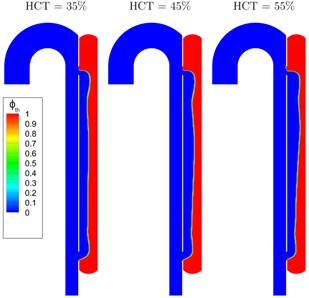
The final state of
thrombus formation is depicted for the three different cases in Figure 9. Based
on the contour for ![]() , this confirms that the qualitatively similar
growth behaviour is reflected in a similar thrombosis of the FL for the
different HCT values.
, this confirms that the qualitatively similar
growth behaviour is reflected in a similar thrombosis of the FL for the
different HCT values.
The results are in agreement with clinical observations, indicating that higher HCT values are correlated with reduced blood clotting and decreasing clot strengths [14-16].
 for different HCT values after 100 cardiac
cycles, at which the growth rate is approaching to zero.
for different HCT values after 100 cardiac
cycles, at which the growth rate is approaching to zero. The current model offers a purely haemodynamic
and rheological explanation of this correlation. At the outset, only the FL
without thrombus is present. The flow rate distributions are very similar at
this point, but the higher value for the haematocrit causes a higher viscosity,
in turn higher wall shear stresses and thus the threshold values ![]() and
and ![]() , respectively, are exceeded in more areas. The
cycle averaged wall shear stresses at this stage are given in Figure 10. The
colour coding facilitates the identification of areas in which
, respectively, are exceeded in more areas. The
cycle averaged wall shear stresses at this stage are given in Figure 10. The
colour coding facilitates the identification of areas in which ![]() exceeds the threshold value of 0.2 Pa, above
which the coagulant production at the wall stops (compare Eq. (14)), which
constrains the growth of thrombus. This effect is enhanced with increasing
haematocrit and results in a slower, delayed and prolonged thrombosis [14].
exceeds the threshold value of 0.2 Pa, above
which the coagulant production at the wall stops (compare Eq. (14)), which
constrains the growth of thrombus. This effect is enhanced with increasing
haematocrit and results in a slower, delayed and prolonged thrombosis [14].
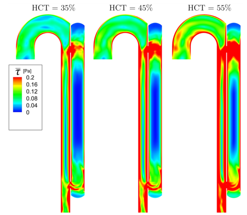
Presumably, the dependence of the shear thinning on the HCT value additionally enlarges the cycle averaged shear stresses. The reason is, that the shear-thinning behaviour of blood causes the velocity profile to be flattened in the vicinity of the FL center line, causing steeper velocity gradients near the wall. This entails higher shear rates towards the wall. The shear thinning effect likewise increases with increasing haematocrit value (cf. Figure 1), such that the velocity profile will be more flattened at higher HCT. The effect of the shear thinning behaviour, however, has not been quantified so far.
The current discussion of course only explains why the current, strongly simplified model of thrombus growth shows a haematocrit dependence, which is in line with experimental observations. If these rheological effects actually cause, or at least contribute to, the reduced blood clotting at high HCT values may only be answered in future research.
8. Conclusions
This paper presents the application of a haemodynamic-based thrombus formation model for studying the haematocrit dependency of FL thrombosis in type B aortic dissection. A rheological model accounting for shear-thinning and a yield stress is applied for the blood flow simulations. Shear rheometric data of human blood was measured by a rheometer. The yield stress was modelled based on data from the literature. Our study predicted a higher probability of complete thrombosis for cases with lower haematocrit values. This is due to an increase in wall shear stress, viscosity and shear rate in the FL with the HCT values. The results are in agreement with clinical observations on blood clotting and suggest that the negative influence of HCT on blood clotting might be due to its rheological effects on blood viscosity and shear thinning behaviour.
9. Limitations
Even though the model equations were implemented for the general 3-dimensional case, the presented problem in this work was only solved in 2-D. The applicability for the 3-dimensional case must be ensured, as well.
Acknowledgements
The authors gratefully acknowledge funding by TU Graz within the LEAD project “Mechanics, Modelling, and Simulation of Aortic Dissection.” Blood rheometry was carried out at the Center of Biomedical Research of the Medical University of Vienna.

References
[1] C.A. Nienaber, R.E. Clough, N. Sakalihasan, T. Suzuki, R. Gibbs, F. Mussa, M.P. Jenkins, M.M. Thompson, A. Evangelista, J.S.M. Yeh, N. Cheshire, U. Rosendahl, and J. Pepper, “Aortic dissection,” Nat Rev Dis Primers., vol. 2, no. 1, 2016. View Article
[2] C. Menichini and X.Y. Xu, “Mathematical modeling of thrombus formation in idealized models of aortic dissection: initial findings and potential applications,” J. Math. Biol., vol. 73, no. 5, pp. 1205–1226, 2016. View Article
[3] T.T. Tsai, A. Evangelista, C.A. Nienaber, T. Myrmel, G. Meinhardt, J.V. Cooper, D.E. Smith, T. Suzuki, R. Fattori, A. Llovet, J. Froehlich, S. Hutchison, A. Distante, T. Sundt, J. Beckman, J.L. Januzzi Jr., E.M. Isselbacher, and K.A. Eagle, “Partial thrombosis of the false lumen in patients with acute type B aortic dissection,” N Engl J Med., vol. 357, no. 4, pp.349–359,2007. View Article
[4] S. Trimarchi, J.L. Tolenaar, F.H.W. Jonker, B. Murray, T.T. Tsai, K.A. Eagle, V. Rampoldi, H.J.M. Verhagen, J.A. van Herwaarden, F.L. Moll, B.E. Muhs, and J.A. Elefteriades, “Importance of false lumen thrombosis in type B aortic dissection prognosis,” The Journal of Thoracic and Cardiovascular Surgery., vol. 145, no. 3, pp. S208–S212,2013. View Article
[5] M. Anand, K. Rajagopal, and K.R. Rajagopal, “A model incorporating some of the mechanical and biochemical factors underlying clot formation and dissolution in flowing blood,” Journal of Theoretical Medicine., vol. 5, no. 3–4, pp. 183–218, 2003. View Article
[6] J.J. Hathcock, “Flow effects on coagulation and thrombosis,” ATVB., vol. 26, no. 8, pp. 1729–1737, 2006. View Article
[7] C.G. Caro, T.J. Pedley, R.C. Schroter, W.A. Seed, and K.H. Parker, “The mechanics of the circulation”, 2009. . View Article
[8] A.L. Fogelson and K.B. Neeves, “Fluid mechanics of blood clot formation,” Annu. Rev. Fluid Mech., vol. 47, no. 1, pp. 377–403, 2015. View Article
[9] C. Menichini, Z. Cheng, R.G.J. Gibbs, and X.Y. Xu, “Predicting false lumen thrombosis in patient-specific models of aortic dissection,” J. R. Soc. Interface., vol. 13, no. 124, pp. 20160759, 2016. View Article
[10]P.J. Carreau, “Rheological equations from molecular network theories,” Transactions of the Society of Rheology., vol. 16, no. 1, pp. 99–127, 1972. . View Article
[11]A. Jafarinia, T.S. Müller, U. Windberger, G. Brenn, and T. Hochrainer, “A study on thrombus formation in case of type B aortic dissection and its hematocrit dependence,” Proceedings of the 6th World Congress on Electrical Engineering and Computer Systems and Science., Avestia Publishing 2020. View Article
[12]E.W. Merrill, “Rheology of blood,” Physiological Reviews., vol. 49, no. 4, pp. 863–888, 1969. View Article
[13]J. Alastruey, N. Xiao, H. Fok, T. Schaeffter, and C.A. Figueroa, “On the impact of modelling assumptions in multi-scale, subject-specific models of aortic haemodynamics,” J. R. Soc. Interface., vol. 13, no. 119, pp. 20160073, 2016. View Article
[14] U. Windberger, Ch. Dibiasi, E.M. Lotz, G. Scharbert, A. Reinbacher-Koestinger, I. Ivanov, L. Ploszczanski, N. Antonova, and H. Lichtenegger, “The effect of hematocrit, fibrinogen concentration and temperature on the kinetics of clot formation of whole blood,” CH., vol. 75, no. 4, pp. 431–445, 2020. View Article
[15]A.S. Jensen, P.I. Johansson, L. Idorn, K.E. Sørensen, U. Thilén, E. Nagy, E. Furenäs, and L. Søndergaard, “The haematocrit – an important factor causing impaired haemostasis in patients with cyanotic congenital heart disease,” International Journal of Cardiology., vol. 167, no. 4, pp. 1317–1321, 2013.View Article
[16] Y. Hayashi, M.-A. Brun, K. Machida, S. Lee, A. Murata, S. Omori, H. Uchiyama, Y. Inoue, T. Kudo, T. Toyofuku, M. Nagasawa, I. Uchimura, T. Nakamura, and T. Muneta, “Simultaneous assessment of blood coagulation and hematocrit levels in dielectric blood coagulometry,” BIR., vol. 54, no. 1, pp. 25–35, 2017. View Article