Journal of Biomedical Engineering and Biosciences (JBEB)
ISSN: 2564-4998

Volume 4 - Year 2017 - Pages 43 - 51
DOI: 10.11159/jbeb.2017.005
Determining Frictional Characteristics of Human Ocular Surfaces by Employing BSG-Starcraft of Particle Swarm Optimization
Sarwo Pranoto1,3, Shingo Okamoto1, Jae Hoon Lee1, Atsushi Shiraishi2, Yuri Sakane2, Yuichi Ohashi2
1Mechanical Engineering Course, Graduate School of Science and Engineering, Ehime University
3 Bunkyo-cho, Matsuyama 790-8577, Japan
c861004y@mails.cc.ehime-u.ac.jp; okamoto.shingo.mh@ ehime-u.ac.jp; lee.jaehoon.mc@ehime-u.ac.jp
2Department of Ophthalmology, Ehime University School of Medicine
Shitsukawa, Toon, Ehime 791-0295, Japan
shiraia@m.ehime-u.ac.jp; y-sakane@ m.ehime-u.ac.jp; ohashi@ m.ehime-u.ac.jp
3Department of Electrical Engineering, Politeknik Negeri Ujung Pandang
Jl. Perintis Kemerdekaan Km. 10, Makassar, Sulawesi Selatan, Indonesia, 90245
sarwo.pranoto@poliupg.ac.id
Abstract - The main purpose of this research is to determine frictional characteristics of human ocular surfaces. A mathematical model for frictional coefficients was proposed. Parameters of the model were determined by a computational algorithm employing BSG (BattleStar Galactica)-Starcraft of PSO (Particle Swarm Optimization). This research also aims to show validities the computational algorithm employing the BSG-Starcraft of PSO and the algorithm employing the genetic algorithm and least-squares method developed in the authors’ previous research. The physical apparatus developed by the authors in the previous research was used to measure the normal forces, frictional forces and velocities of the probe on eye surfaces of healthy subjects simultaneously. Then, the frictional characteristic curves of human ocular surfaces were calculated by using the present and previous computational algorithms. Finally, both computational algorithms were validated by comparing both results on the frictional characteristics of cornea and bulbar conjunctiva. The authors have succeeded in determining the frictional characteristics of human ocular surfaces.
Keywords: BSG-Starcraft of PSO, Frictional coefficient, Frictional characteristic, Human ocular surface.
© Copyright 2017 Authors This is an Open Access article published under the Creative Commons Attribution License terms. Unrestricted use, distribution, and reproduction in any medium are permitted, provided the original work is properly cited.
Date Received: 2017-02-22
Date Accepted: 2017-10-29
Date Published: 2017-12-04
1. Introduction
In recent years, dry eye syndrome has been recognized as common health problems that cause patients visiting ophthalmologists. Dry eye syndrome may cause deterioration of quality of life and vision. Therefore, many researches on dry eye syndrome have been performed. S. Patel et al. [1] reported that during the use of visual displays, people tend to reduce their blinking rate and the stability of tear film.
In addition, M. Uchino et al. [2] stated that dry eye syndrome has a significant influence on patients’ quality of life. Moreover, M. Uchino et al. [3] concluded that dry eye syndrome decreases attendance rate in workplaces of people using visual displays in Japan.
In addition, the increasing use of contact lenses may cause the increasing dry eye syndrome. M. Guillon et al. [4] reported that some 43% of volunteers wearing soft contact lenses in Contact Lens Research Consultants, London, U.K were recognized have dry eye symptoms. Their study concluded that persons wearing contact lenses are more vulnerable to get dry eye syndrome than persons without contact lenses.
Furthermore, researchers have shown an increased interest in mechanical friction on a human ocular surface. H. Pult et al. [5] discussed the friction between upper eyelid and cornea or between upper eyelid and surfaces of a contact lens during spontaneous blinks. Besides, H. Pult et al. [6] investigated correlations between the blink frequency and the type of blink, and between the dry eye symptoms and the lid-parallel conjunctival folds. Moreover, I. Cher [7] studied disorders on ocular surfaces that may be caused by mechanical friction or deterioration of a function of lubricity within the eyes. In addition, the authors of this paper [8] assessed a newly developed eyelid pressure measurement system using a tactile pressure sensor. This system is used to evaluate the pressure of the eyelids on the ocular surface in normal and diseased eyes.
Furthermore, measurements of frictional coefficients of human ocular surfaces have been conducted by some researchers. T. Wilson et al. [9] performed the measurements of frictional coefficients on ocular surfaces of twenty eight humans. This report stated that the frictional coefficients of human ocular surfaces lie between 0.006 and 0.015. Recently, the authors of this paper [10] developed the frictional coefficients of human ocular surfaces have been measured using the physical apparatus. In their research, the computational algorithm combining the genetic algorithm and least-squares method was also developed for measuring the frictional coefficients of human ocular surfaces.
On the other hand, many researches have been conducted to solve optimization problems using some algorithms such as PSO and genetic algorithm. Some researchers have examined the effectiveness of PSO and genetic algorithm. S. Panda et al. [11] compared the performance of both algorithms in order to solve the stabilities of a power system. They reported that both algorithms could be used in optimizing parameters of the controller of FACTS (Flexible Alternating Current Transmission System). In addition, R. Hassan et al. [12] examined the computational efficiency of both genetic algorithm and PSO to find solutions of optimization test functions. In their study, it is reported that the PSO is more efficient than the genetic algorithm.
While, among many variants of PSO, S. Salmon [13] developed the BSG-Starcraft of PSO and evaluated its performance by solving some optimization test functions. The idea of the BSG-Starcraft of PSO came from the movie of BattleStar Galactica and a video game Starcraft. Then, the BSG-Starcraft of PSO has been used to solve optimization problems. For example, D. Chamoret et al. [14] implemented the BSG-Starcraft of PSO to minimize the thermal residual stresses (TRS) of the unidirectional ceramic matrix composites (CMCs).
Although many researches have been interested in mechanical friction of human ocular surfaces, the frictional characteristics of human ocular surfaces have not been clarified. In addition, to best our knowledge, no studies exist on mechanical friction of human ocular surfaces which employing the BSG-Starcraft of PSO to determine the frictional characteristics of human ocular surfaces.
In the present study, the physical apparatus developed by the authors in the previous research was used to measure the normal forces, frictional forces and velocities of the probe on eye surfaces of healthy subjects simultaneously. The computational algorithm employing the BSG-Starcraft of PSO was developed to determine the frictional characteristics of human ocular surfaces. The frictional characteristic curves of cornea and bulbar conjunctiva were calculated by using both the algorithm employing the BSG-Starcraft of PSO and the algorithm employing the genetic algorithm developed by the authors’ previous research. In addition, the validation of the computational algorithms was conducted by comparing the frictional characteristics of cornea and bulbar conjunctiva obtained by the BSG-Starcraft of PSO and those obtained by the genetic algorithm.
2. Frictional Coefficients of Human Ocular Surface
2.1. Physical Apparatus for Measuring the Frictional Coefficients
In the field of mechanical engineering, it is generally accepted that the Hersey Number can be used to identify the frictional coefficients on journal bearings. The Hersey Number [15] is expressed by

Where η, ω, and p denote the viscosity of lubricating oil, the rotational speed of a shaft, and the pressure of lubricating oil behind the location of the minimum separation between the shaft and the bearing, respectively.
In this research, it is considered that the frictional coefficient, µ of a human ocular surface is related to the viscosity, η of tear fluid, the velocity, Vn of nictation, and the palpebral pressure, P. Then, the physical apparatus that can measure the moving velocity, V of the probe, the normal force, N and the frictional force, F was developed by the research group of authors [10].
Figure 1 shows the moving directions of the probe in the physical apparatus on the left eye. The probe is contacted on the human ocular surface by moving it in the Z direction. Then the normal force, N, the frictional force, F and the moving velocity, V of the probe are measured by moving the probe in the X direction.
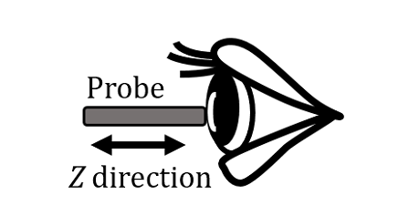
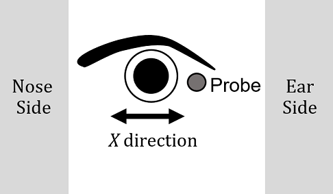
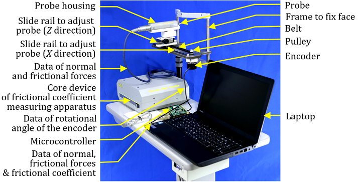
Figure 2 shows the frictional coefficient measuring unit assembly including the frictional coefficient measuring apparatus and the device to measure the moving velocity of the probe. The frictional coefficient measuring unit was used to measure the normal force, N and the frictional force, F acquired by the probe. The normal force, N and the frictional force, F were collected by the core device of the frictional coefficient measuring apparatus that is connected to a laptop. The device developed by the authors was used to measure the moving velocity, V of the probe. The device consists of a frame to fix a face, an encoder, two pulleys, a belt, a probe housing, a microcontroller and a laptop. The encoder is connected to the microcontroller in order to convert the angular velocity, ωp of the pulleys to the corresponding the moving velocity, V of the probe connected to the belt to rotate the pulleys.
2.2. Mathematical Model for Frictional Coefficients
In a normal eye, a tear layer exists between the ocular surface and the eyelid, whereas in a dry eye, some areas of the surfaces directly contact each other. Thus, the frictional coefficient, µ of a human ocular surface is considered to be within the range of fluid lubrication when the surfaces are fully separated by the tear layer and considered to be within the range of mixture lubrication when the ocular surface is dry.
In this research, a new number, X that is capable of calculating the frictional coefficient, µ of the human ocular surface given by equation (2) is proposed as follows:

Where parameters, p1, p2 and p3 denote arbitrary real numbers.
Then the authors propose the mathematical model describing the frictional coefficient, µ of the human ocular surface by incorporating the proposed number, X as follows:
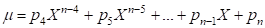
Where parameters, p4, p5, … and pn also denote arbitrary real numbers. In this paper, it is assumed that η is constant and equal to 1, in other words p1 = 0.
3. BSG-Starcraft of PSO
3.1. Parameters in Frictional Characteristic Curve of Human Ocular Surface Using BSG-Starcraft of PSO
In this research, determining parameters p1, …, pn in Eq. (2) and Eq. (3) was treated as an optimization problem. As compared with genetic algorithm, PSO has been proven to have some advantages. The PSO is simpler for composition of an algorithm, faster for computational speed, and fewer for the number of parameters than the genetic algorithm. Therefore, in this paper, the PSO was applied to solve optimal values for the parameters. Then, a computational algorithm employing the BSG-Starcraft of PSO was developed to identify the parameters, p1, …, pn in Eq. (2) and Eq. (3). The computational algorithm consists of several steps.
The first step is the initialization of positions, velocities and inertia weights of all particles in the swarm. The position and
velocity of particle i at iteration j in the n-dimensional search space were denoted as ![]() and
and![]() respectively.
respectively.
The initial positions, ![]() and velocities,
and velocities, ![]() of all particles were randomly
generated within pre-defined ranges as expressed in Equations (4) and (5).
of all particles were randomly
generated within pre-defined ranges as expressed in Equations (4) and (5).

Here ![]() and
and ![]() denote the lower and upper bounds on x,
respectively.
denote the lower and upper bounds on x,
respectively.

Here ![]() and
and ![]() the lower and upper bounds on v,
respectively.
the lower and upper bounds on v,
respectively.
While the inertia weight, ![]() was
calculated as follows:
was
calculated as follows:
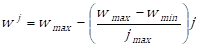
Where ![]() and
and ![]() denote the minimum and maximum inertia weights. In this research,
denote the minimum and maximum inertia weights. In this research, ![]() and
and ![]() were set to 0.4 and 0.9, respectively.
were set to 0.4 and 0.9, respectively.
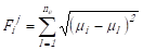
The second step is the evaluation of the objective function. The objective function, ![]() of particle i at iteration j was given by:
of particle i at iteration j was given by:
 (i = 1 ~
 Here ![]() ,
, ![]() and
and ![]() denote the actual experimental value of frictional coefficient of the human ocular surface, the
number of experimental values and the number of particles in a swarm,
respectively. In this research, the value of the objective function,
denote the actual experimental value of frictional coefficient of the human ocular surface, the
number of experimental values and the number of particles in a swarm,
respectively. In this research, the value of the objective function, ![]() was
minimized by the BSG-Starcraft of PSO algorithm.
was
minimized by the BSG-Starcraft of PSO algorithm.
The third step is the determination of the personal best position of particle i, ![]() and the best global position in the current
swarm,
and the best global position in the current
swarm, ![]() . The personal best position of particle i,
. The personal best position of particle i,
![]() is determined by the smallest value of the objective function,
is determined by the smallest value of the objective function, ![]() obtained
by the particle i at all previous iterations. The personal best position of particle i,
obtained
by the particle i at all previous iterations. The personal best position of particle i, ![]() that has
the smallest value of the objective function among the others is determined as
that has
the smallest value of the objective function among the others is determined as ![]() .
.
The fourth step is the selection of the best global position in the current swarm, ![]() as the carrier,
as the carrier, ![]() . In each iteration, the
carrier,
. In each iteration, the
carrier, ![]() is used to send some new
particles called raptors,
is used to send some new
particles called raptors, ![]() with
the probability 0.9. The objective function,
with
the probability 0.9. The objective function, ![]() of
raptor k at iteration j is evaluated using formula as expressed
in Equation (8).
of
raptor k at iteration j is evaluated using formula as expressed
in Equation (8).
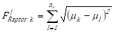 (k = 1 ~
 Here ![]() denotes the number of raptors
in each iteration. In this research,
denotes the number of raptors
in each iteration. In this research, ![]() was set to
20.
was set to
20.
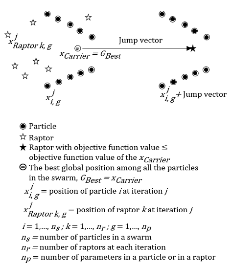
Figure 3 shows the schematics of raptors exploring the space. A jump
vector, namely Jump is defined when there is one raptor reaches best
position than the best global position in the current swarm,![]() Consequently, the swarm jumps to the new position by the translation of
the vector Jump. The carrier,
Consequently, the swarm jumps to the new position by the translation of
the vector Jump. The carrier, ![]() position is now the raptor which has the best position.
Therefore, the
position is now the raptor which has the best position.
Therefore, the ![]() and
and ![]() are updated due to the new position of the swarm.
are updated due to the new position of the swarm.
In the fifth and sixth steps, the velocity and position of particle i are updated using Equations (9) and (10), respectively.
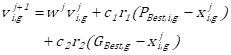
Here ![]() and
and ![]() denote the self confidence factor and the swarm confidence factor,
respectively. In this research,
denote the self confidence factor and the swarm confidence factor,
respectively. In this research, ![]() and
and ![]() were set equal to 2. The
were set equal to 2. The ![]() and
and ![]() denote the random numbers uniformly distributed in the range (0, 1).
denote the random numbers uniformly distributed in the range (0, 1).
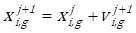
Figure 4 shows the updating velocity and position of a particle. In order to update the velocity, ![]() of the particle i expressed in Eq. (9), the best global position,
of the particle i expressed in Eq. (9), the best global position, ![]() in the current swarm and the personal best position,
in the current swarm and the personal best position, ![]() of the particle i are combined with
of the particle i are combined with ![]() ,
, ![]() ,
, ![]() ,
, ![]() and
and ![]() . The position,
. The position, ![]() of the particle i in the next iteration is affected by the
current velocity,
of the particle i in the next iteration is affected by the
current velocity, ![]() of the particle i, the best global position,
of the particle i, the best global position, ![]() in the current swarm and the personal best position,
in the current swarm and the personal best position, ![]() of the particle i.
of the particle i.
3.2. Procedure for Determining Parameters in Frictional Characteristic Curve of Human Ocular Surface Using BSG-Starcraft of PSO
The procedure for determining parameters in the frictional characteristic curve of the human ocular surface using the BSG-Starcraft of PSO is given by the pseudo-code as follows:
- Randomly initialize
 ,
,  and
and  of all particles
 - Evaluate the objective function of all particles,

- Determine the personal best position of particle i,

- Determine the best global position in the current swarm,

- while j ≤
 do
do - for i =1 to
 do
do - Set the
 as the carrier,
- Randomly create
 raptors, with a probability = 0.9
 - Evaluate the objective function,
 of raptor k at iteration j
 - if
 ≤
≤  then
then - Set the jump vector as
Jump = - and jump the swarm to the new position
 - Evaluate the objective function for the swarm at the new position
- Else
- Evaluate the objective function of the swarm at the original position
- end if
- Update the

- Update the
- Update the velocity of particle i according to Eq. (9)
- Update the position of particle i according to Eq. (10)
- end for
- end while
4. Data Measured by Physical Apparatus
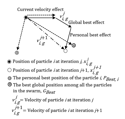
Figure 5 shows the examples of cornea’s data measured by the physical apparatus. Time history responses of normal forces, N, frictional forces, F and displacements, d of the probe were measured at the same time using the physical apparatus.
In this experiment, the normal forces, N were applied to the cornea within the range of 9.33 × 10⁻² [N] to 2.63 × 10⁻¹ [N]. As for the displacements, d, of the probe, they were measured by the encoder. The displacements, d were controlled to be within the range of 2.00 × 10⁻³ [m] to 4.25 × 10⁻³ [m]. As for the normal forces, N and the frictional forces, F, their average values were calculated from each measured data.
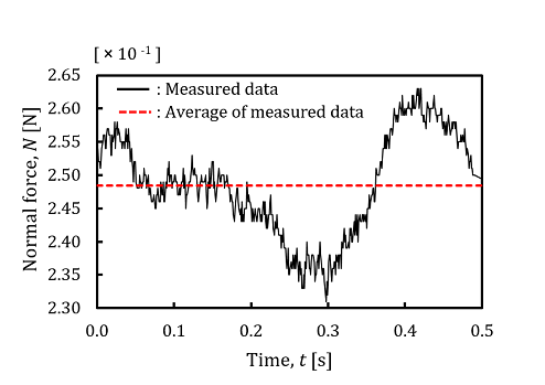
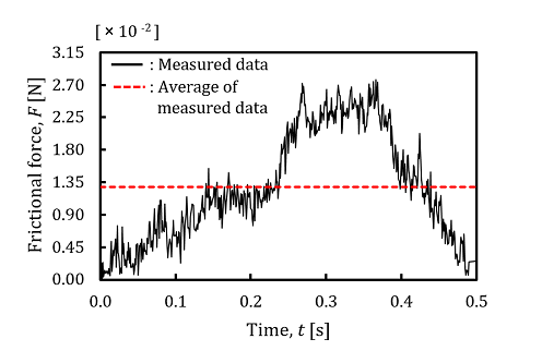
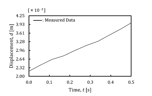
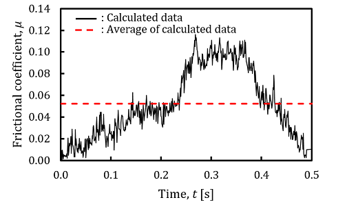
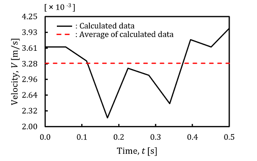
Figure 6 shows the examples of cornea’s results calculated by using the measured data. The frictional coefficients, µ were calculated by using the measured the normal forces, N and the frictional forces, F. The velocities, V of the probe were calculated by using the measured displacements, d of the probe. The average values of the frictional coefficients, µ and the velocities, V were calculated in order to determine the frictional characteristics of human ocular surface.In this experiment, the average values of the frictional coefficients, µ varied within the range of 0.04 to 0.11. The average values of the velocities, V of the probe varied within the range of 2.04 × 10⁻³ [m/s] to 3.98 × 10⁻³ [m/s].
The calculated results on the bulbar conjunctiva were similar to those of the cornea. The average values of the frictional coefficients, µ varied within the range of 0.04 to 0.13. The average values of the velocities, V of the probe varied within the range of 1.81 × 10⁻³ [m/s] to 3.07 × 10⁻³ [m/s].
4.1. Frictional Characteristic Curves of Human Ocular Surface Calculated by Using BSG-Starcraft of PSO
In this research, the data measured from healthy subjects were used to determine the frictional characteristic curves of human ocular surface by using the BSG-Starcraft of PSO.
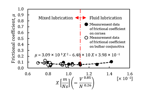
Figure 7 shows the examples of frictional characteristic curves calculated by using the BSG-Starcraft of PSO. The calculated frictional coefficient, µ of human ocular surface were plotted as the function of X, based on the values of V and N.
Figure 7 (a) shows the frictional characteristic curve of cornea and bulbar conjunctiva in mixed and fluid lubrication regions. These data were obtained from one of the healthy subjects. The BSG-Starcraft of PSO was implemented by setting the number, ![]() = 20 of particles in a swarm. The parameters,
= 20 of particles in a swarm. The parameters, ![]() = 0.85 and
= 0.85 and ![]() = 0.26 indicate the values obtained when the objection function became the best value,
= 0.26 indicate the values obtained when the objection function became the best value, ![]() = 0.103. The best objective function value,
= 0.103. The best objective function value, ![]() achieved
within the maximum iteration number,
achieved
within the maximum iteration number, ![]() = 200. As
for this subject, the results on the cornea revealed that the frictional
coefficients fall within both the mixed lubrication and the fluid one. Then,
the results on the bulbar conjunctiva revealed that the frictional coefficients fall within only the mixed lubrication.
= 200. As
for this subject, the results on the cornea revealed that the frictional
coefficients fall within both the mixed lubrication and the fluid one. Then,
the results on the bulbar conjunctiva revealed that the frictional coefficients fall within only the mixed lubrication.
When the measurement on Figure 7 (a) was carried out, the measurement on the cornea was firstly conducted, then followed by the measurement of the bulbar conjunctiva. Thus, the measurement data on the cornea showed that they were in both wet and dry conditions. While the measurement data on the bulbar conjunctiva showed that they were in only dry condition.
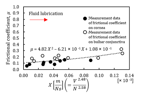
Figure 7 (b) shows the frictional characteristic curve of cornea and bulbar conjunctiva in fluid lubrication region. These data were obtained from another healthy subject. The BSG-Starcraft of PSO was implemented
by setting the number, ![]() = 40 of particles in a swarm. The parameters,
= 40 of particles in a swarm. The parameters, ![]() = 2.48 and
= 2.48 and ![]() = 2.58 indicate the values obtained when the objective function became the best value,
= 2.58 indicate the values obtained when the objective function became the best value, ![]() = 0.202. The best value,
= 0.202. The best value, ![]() =
0.202 achieved within the maximum iteration number,
=
0.202 achieved within the maximum iteration number, ![]() = 200. The results on both the
cornea and the bulbar conjunctiva revealed that the frictional coefficients
fall within only the fluid lubrication.
= 200. The results on both the
cornea and the bulbar conjunctiva revealed that the frictional coefficients
fall within only the fluid lubrication.
When the measurement on Figure 7 (b) was carried out, the measurement on the cornea was firstly conducted, then followed by the measurement of the bulbar conjunctiva. As for this subject, the measurement data on both the cornea and the bulbar conjunctiva showed that they were in only wet condition.
4.2. Comparison of Frictional Characteristic Curves of Human Ocular Surface Calculated by Computational Algorithms Employing both BSG-Starcraft of PSO and Genetic Algorithm
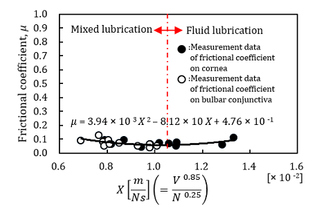
Figure 8 shows the examples of frictional characteristic curves calculated by using the genetic algorithm. The calculated frictional coefficients, µ of human ocular surface were plotted as the function of X, based on the values of V and N.
Figure 8 (a) shows the frictional characteristic curve of cornea and bulbar conjunctiva in mixed and fluid lubrication regions. These data used in Figure 8 (a) are the same ones as Figure 7 (a). The parameters ![]() = 0.85 and
= 0.85 and ![]() = 0.25 indicate the values obtained by using the genetic algorithm.
= 0.25 indicate the values obtained by using the genetic algorithm.
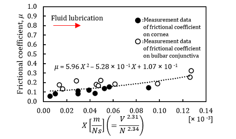
Figure 8 (b) shows the frictional characteristic curve of cornea and bulbar conjunctiva in fluid lubrication region. These data used in Figure 8 (b) are the same ones as Figure 7 (b). In Figure 8 (b), the frictional characteristic curve of cornea and bulbar conjunctiva fall within only fluid lubrication region. The parameters ![]() = 2.31 and
= 2.31 and ![]() = 2.34 indicate the values
determined by using the genetic algorithm.
= 2.34 indicate the values
determined by using the genetic algorithm.
Despite using the different methods, namely the BSG-Starcraft of PSO and the genetic algorithm, the frictional characteristic curves of human ocular surface calculated by the BSG-Starcraft of PSO have the similar characteristics as those calculated by the genetic algorithm.
It is generally said that both the BSG-Starcraft of PSO and the genetic algorithm cannot find one determinative solution because both methods are evolutionary algorithms. However, frictional characteristic curves calculated by the BSG-Starcraft of PSO have the similar characteristics as those calculated by the genetic algorithm. These results represent that the frictional characteristic curves calculated by the BSG-Starcraft of PSO and the genetic algorithm are reasonable.
5. Conclusion
The summary of the results is shown below.
- The computational algorithm employing BSG-Starcraft of PSO for determining the frictional characteristics of the human ocular surface was developed.
- Frictional characteristic curves of the human ocular surface have been calculated by using both the algorithm employing the BSG-Starcraft of PSO and the algorithm employing the genetic algorithm developed by the authors’ previous research.
- The validities of the both computational algorithm employing the BSG-Starcraft of PSO and the algorithm developed in the previous work employing the genetic algorithm and least-squares method were shown by comparing the both results of the frictional characteristics of the human ocular surfaces. It can be concluded that both the computational algorithms employing the BSG-Starcraft of PSO and the genetic algorithm are reasonable for determining the frictional characteristics of the human ocular surfaces.
References
[1] S. Patel, R. Henderson, L. Bradley, B. Galloway, and L. Hunter, “Effect of visual display unit use on blink rate and tear stability,” Optometry & Vision Science, vol. 68, no. 11, pp. 888-892, 1991. View Article
[2] M. Uchino, and D. A. Schaumberg, “Dry eye disease: impact on quality of life and vision,” Current ophthalmology reports, vol.1, no. 2, pp. 51-57, 2013. View Article
[3] M. Uchino, Y. Uchino, M. Dogru, M. Kawashima, N. Yokoi, A. Komuro, Y. Sonomura, H. Kato, S. Kinoshita, D. A. Schaumberg, and K. Tsubota, “Dry eye disease and work productivity loss in visual display users: the Osaka study,” American journal of ophthalmology, vol. 157, no. 2, pp. 294-300, 2014. View Article
[4] M. Guillon, and C. Maissa, “Dry eye symptomatology of soft contact lens wearers and nonwearers,” Optometry & Vision Science, vol. 82, no. 9, pp. 829-834, 2005. View Article
[5] H. Pult, S. G. Tosatti, N. D. Spencer, J. M. Asfour, M. Ebenhoch, and P. J. Murphy, “Spontaneous blinking from a tribological viewpoint,” The ocular surface, vol. 13, no. 3, pp. 236-249, 2015. View Article
[6] H. Pult, B. H. Riede-Pult, and P. J. Murphy, “The relation between blinking and conjunctival folds and dry eye symptoms,” Optometry & Vision Science, vol. 90, no. 10, pp. 1034-1039, 2013. View Article
[7] I. Cher, “Blink-related microtrauma: when the ocular surface harms itself,” Clinical & Experimental Ophthalmology, vol. 31, no. 3, pp. 183-190, 2003. View Article
[8] E. Sakai, A. Shiraishi, M. Yamaguchi, K. Ohta, and Y. Ohashi, “Blepharo-tensiometer: new eyelid pressure measurement system using tactile pressure sensor,” Eye & Contact Lens, vol. 38, no. 5, pp. 326-330, 2012. View Article
[9] T. Wilson, R. Aeschlimann, S. Tosatti, Y. Toubouti, J. Kakkassery, and K. O. Lorenz, “Coefficient of friction of human corneal tissue,” Cornea, vol. 34, no. 9, pp. 1179-1185, 2015. View Article
[10] S. Okamoto, S. Pranoto, Y. Ohwaki, J. H. Lee, A. Shiraishi, Y. Sakane, K. Ohta, Y. Ohashi, “Development of a Physical Apparatus and Computational Program Employing a Genetic Algorithm and Least-Squares Method for Measuring the Frictional Coefficient of the Human Ocular Surface,” in Proceedings of 3rd International Conference on Biomedical Engineering and Systems (ICBES'16), Budapest, Hungary, 2016. View Article
[11] S. Panda, and N. P. Padhy, “Comparison of particle swarm optimization and genetic algorithm for FACTS-based controller design,” Applied soft computing, vol. 8, no. 4, pp. 1418-1427, 2008. View Article
[12] R. Hassan, B. Cohanim, O. De Weck, and G. Venter, “A comparison of particle swarm optimization and the genetic algorithm,” in Proceedings 46th AIAA/ASME/ASCE/AHS/ASC Structures, Structural Dynamics and Materials Conference, p. 1897, 2005. View Article
[13] S. Salmon, “Particle Swarm Optimization in Scilab ver 0.1-7,” Performance evaluations, 2011.
[14] D. Chamoret, S. Salmon, N. Di Cesare, and Y. J. Xu, “BSG-Starcraft radius improvements of particle swarm optimization algorithm: An application to ceramic matrix composites,” in International Conference on Swarm Intelligence Based Optimization, Springer International Publishing, pp. 166-174, 2014. View Article
[15] B. J. Hamrock, S. R. Schmid, and B. O. Jacobson, Fundamentals of Fluid Film Lubrication. New York: Marker Dekker, Inc., 2004.