Journal of Biomedical Engineering and Biosciences (JBEB)

ISSN: 2564-4998

1. Introduction

Sleep apnea (SA) is generally expressed as not breathing for at least 10 seconds during the sleep. It is an under-diagnosed sleep disorder and is a fatal risk factor. SA is associated with high risks of hypertension, stroke and also with increased mortality rates [1]. Approximately 14% of men and 5% of woman in United States are suffering from OSA syndrome and incidence rate is increasing worldwide [2]. Hypopnea can be defined as 50% decrease in airflow accompanied by 4% oxygen desaturation for at least 10 seconds during the sleep. In a sleep study, the severity level of OSA is measured by the number of apnea and hypopnea events per hour during sleep; known as the apnea-hypopnea index (AHI). A subject having clinical symptoms such as excess daytime sleepiness and impaired cognition in addition to AHI greater than 5, is diagnosed as an OSA patient [3]. AHI is usually calculated through overnight polysomnography (PSG) recorded from suspected OSA patients, in sleep study laboratories. Overnight polysomnography (PSG) is the gold standard method for diagnosis of OSA [4]. PSG requires recordings and monitoring of multi-parameter biophysiological signals, including EEG, ECG, respiratory effort, nasal airflow and oxygen saturation (SpO₂). These recorded signals are then analyzed by sleep specialists for final diagnosis of the apnea syndrome. SA is generally characterized by pauses in breathing or shallow breathing when the soft tissue in the rear of the throat collapses and closes during whole night sleep [5]. A slow respiratory rate caused by the blockage in the airway, results with less supply of oxygen delivered from the lungs to heart and body. Without breathing (or shallow breathing), CO₂ level in the blood begins to elevate and the patient tries to wake up feeling a choke. There are two commonly faced types for apnea: Obstructive sleep apnea (OSA) and Cental sleep apnea (CSA). In OSA, the airflow through nose stalls for a period of time and but the brain struggles with the body to breath. Snoring, having trouble getting up in the morning, depression, headaches in the morning and night sweats may be given as symptoms for OSA. In CSA case, brain is not able to send stimulus to muscular system to resume breathing. Compared to the OSA, snoring is generally not observed with central sleep apnea. Being very tired during the day, having too much headaches and repeatedly waking up during the night are the general symptoms for CSA. There are two devices to overcome apnea syndrome: continuous positive airway pressure (CPAP) and bilevel positive airway pressure (BiPAP). Both devices provide positive airway pressure and contribute to the patient to get more air in and out of the lungs. However, the main difference among them is BiPAP applies higher pressures during inspiration than expiration [6].

There are many studies to detect apnea episodes using PSG recordings. Some of them focus on using ECG signals to detect OSA [7,8]. SA is defined as not or shallow breathing during sleep, for this reason it is more accurate to predict apnea by nasal airflow signal. Han et al. proposed a method to detect apneic events based on second derivatives of the respiratory signal [9]. In another study, Yadollahi and Moussavi developed a fully automatic acoustic method to detect apnea and hypopnea events [10]. Only tracheal breathing sounds and blood oxygen saturation level are used in the proposed method and results with high sensitivity and specificity are obtained. Kim et al. proposed a novel R wave detection algorithm to analyse the heart rate variability (HRV) of obstructive sleep apnea patients [11]. As a measure of apnea classification accuracy, the method correctly classified 99.7% of the evaluation database. Some other recent works have focused on apnea syndrome diagnosis, by using nonlinear measures of airflow signal [12]. In this study, an early warning system is proposed to predict OSA episodes 30 seconds earlier by extracting time-series features of OSA periods and regular respiration. A device that records the nasal airflow signal of the patient throughout the night and runs the proposed algorithm may be a useful approach for urgent pre-intervention. In this wise, it will be possible to warn the patient before apnea episodes even occur.

2. Fully Automatic Sleep Apnea Detection

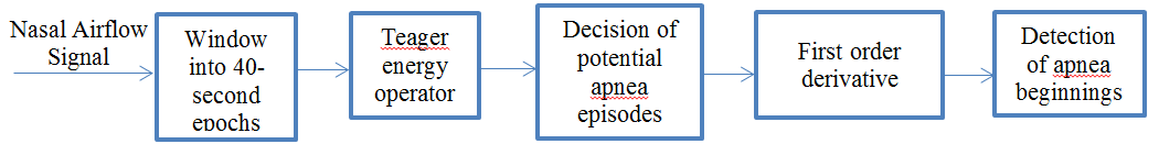
Sleep apnea is the syndrome of pause in breathing during sleep longer than 10 seconds. Our data set has nasal respiratory airflow signals of 13 patients sampled at 32 Hz for an overnight sleep recorded at a sleep study laboratory in hospital. Each of these recordings has duration around 7-8 hours. Nasal airflow signal is first divided into 40 seconds segments (epochs). Every 40-second signal is evaluated independently in terms of energy by using Teager Energy Operator. Epochs containing potential apnea episodes are determined by changes in the energy level. Then, first order derivative approach is applied to the nasal airflow signal episodes, previously labelled as potential apnea candidate. This approach ensures to determine apnea episode beginning precisely. Figure 1 shows the general schematics of the apnea detection algorithm used in this study.

2.1. Nasal Airflow Signal Data

Nasal airflow data is recorded in sleep laboratories belongs to 13 patients of an overnight sleep. Recordings have 7-8 hours of sleep data and airflow signal is sampled at 32 Hz. All of the nasal airflow signal data of all patients are given as an input to the algorithm. A 7-8 hour long signal is first divided into 40-second long epochs to visualize and analyse easier. Each patient data will have around 650 independent epochs each lasts 40 seconds.

2.2. Windowing

It is difficult to detect not only a 10-second apnea episode using an 8-hour nasal airflow signal, but also visualize in shorter intervals. For this reason we divided the nasal airflow signal into 40-second epochs. Each epoch is analyzed independently. The purpose of this independent calculation is to minimize the effects of incorrect samples caused by possible movement of the patient or the transducer dislocation during the sleep. Then every epoch is divided into two distinct 20 second parts (first half and second half) and the energy of each segment is calculated by Teager Energy Operator.

The energy levels of the two 20 second long signals are compared with respect to total energy of the epoch, whether the ratio of average energies is < 0.25 (or > 4) or not. The segments that have less than one quarter of average energy than the average energy of the epoch are marked as potential apnea episodes. Two potential apnea candidate segments are shown in Figure 2 and Figure 3 is an output of the detection algorithm. It can be easily seen that in Figure 2 the patient could not breathe for longer than 10 seconds. On the other hand, mislabelled epoch is detected as potential apnea episode in Figure 3, where there is actually no problem in respiration.

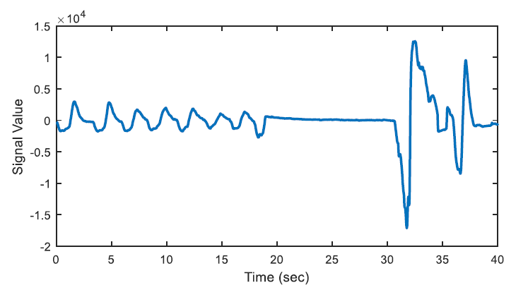
In Figure 2, there happens a pause, up to almost 13 seconds on breathing during the second half of the epoch. On the other hand, the total energy of the epoch is four times greater than the energy of one of the 20-second segments.

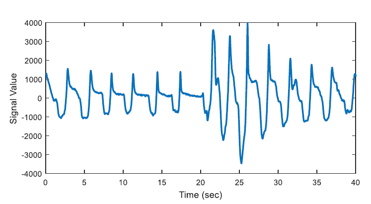
In Figure 3, the epoch is detected as apnea candidate as there happens four times energy difference between the 20-second segments and the total energy of the epoch. It can be seen that there does not occur any apnea syndrome during the epoch. In order to eliminate the mislabelled regions, first order derivative is applied for the next step.

2.3. First Order Derivative Approach

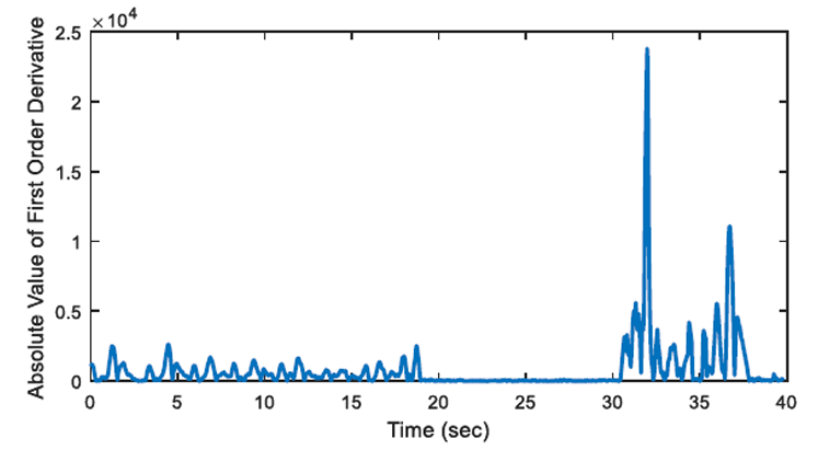
The aim of first order derivative approach is to eliminate mislabelled epochs like in Figure 2.b. In this part, the derivatives of the epochs are calculated. The first order derivative of every 8-sample interval (0.25 seconds for sampling frequency of 32 Hz) is obtained (Figure 4) and compared with a designated threshold value. If the interval length for the derivation is chosen longer, the error in detected apnea beginning precisely increases. Obviously, smaller values may cause other inaccuracies in calculation; considering that nasal airflow signal is not highly deviating. The samples below the threshold value are marked (Figure 5) and they are checked whether there is a segment, composed of consecutive samples, that lasts longer than 10 seconds. If not, these samples are removed from the list of the potential apnea episodes. Moreover, the outputs for the epochs which are labelled incorrectly (like an example in Figure 3) will also be eliminated because of not containing any 10-second long apnea episodes. In this manner, small deviation values which exist for longer than 10 seconds are detected as apnea event and the initial sample value (marked value) for every apnea periods in the whole signal is stored by examining every potential apnea epochs (Figure 6).

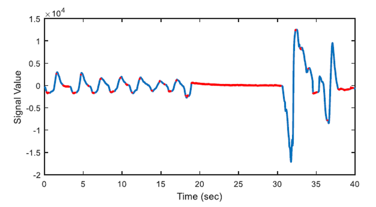
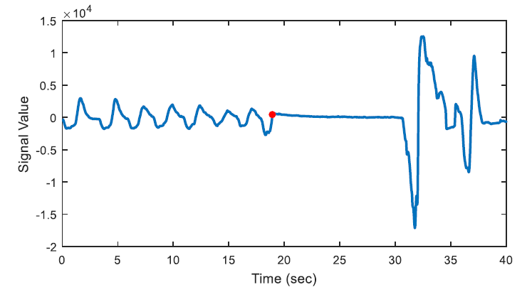
The output of the first order derivative approach is a single sample value that determines and marks the beginning of the sleep apnea episode. It does not include any other data about the duration of the apnea and it will only be used for distinguishing a time interval labelled as pre-apnea.

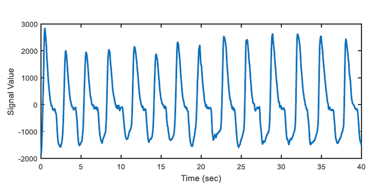
After the apnea detection process is accomplished, regular breathing intervals are detected by using similar approach. An example of automatically detected regular air flow (regular breathing) is shown as an example in Figure 7.

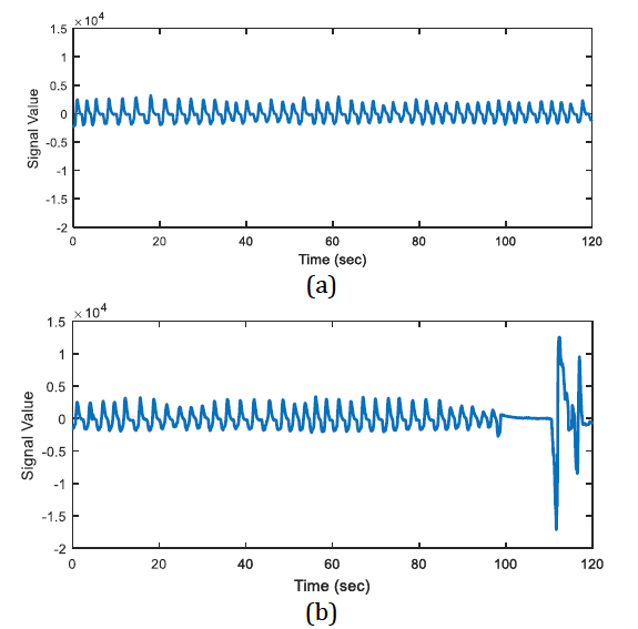
In the algorithm at the end of this section, OSA segments are automatically detected by the developed algorithm and beginning time of these segments are also marked automatically. 347 apnea episodes are detected by analysing all of the nasal airflow signal data of 13 patients. Then regular breathing segments are selected from the remaining respiration signal where OSA segments labelled as "pre-apnea" are removed from the original recording. Labelled OSA and regular breathing segments will be used as training inputs to learning algorithm. 347 regular breathing episodes are extracted to avoid any positive or negative bias in prediction (learning) section. If the number of selected regular breathing episodes is comparably less than the number of pre-apnea segments, learning algorithms will tend to give the output with "apnea bias". In a case where there are 300 pre-apnea and 100 regular breathing training samples, there may be 75% accuracy, by just labelling all test samples as "pre-apnea". To avoid this situation, training and test data set will be selected as containing 50% pre-apnea episodes and 50% regular breathing episodes. With the help of learning algorithms, discussed in the following chapters, the system will be able to predict whether a new signal has an OSA warning or not. As Figure 8 indicates there is not much difference in nasal airflow signals in the means of breathing period or amplitude. Both pre-apne and regular breathing intervals appear similar.

3. Prediction Algorithm

There are two different classes of input, used for prediction: Pre-apnea and regular breathing. Pre-apnea interval is a 1 minute nasal airflow signal which begins 90 seconds before apnea occurs. The beginnings of apnea segments, automatically marked by apnea detection algorithm, are used to extract the pre-apnea interval. By this way, pre-apnea and apnea segments are disaggregated from each other by 30 seconds margin to minimize the pre-effects of apnea. Similarly, 1 minute signal intervals are extracted starting 90 seconds prior to healthy respiration, representing regular breathing. All of the regular breathing intervals, having shallow breathing for at most 2 seconds, are detected and sufficient number of these intervals are chosen randomly to be processed. By this way, it is intended to predict a possible apnea episode and alert before patient faces OSA, by having significant amount of time for processing. Time-series features of both classes are calculated and given as input features to learning algorithms. 347 pre-apnea intervals are extracted for each of 347 marked apnea segments. In order to decrease possible bias in the classification process, 347 regular breathing intervals are selected randomly, having a total of 694 input signals. Pre-apnea and regular breathing intervals are obtained from 13 patients to eliminate any personal effects among individuals.

3.1. Features

In this study only time-series features are considered and used. Most popular features like mean, variance, minimum, maximum, median values of signals are used not only for the original signal but also implemented for the power and derivative of the signal. In addition to these 15 features; minimum, maximum, average inspiration/expiration amplitudes and durations of nasal airflow signal are also extracted for each of 694 signal intervals (pre-apnea and regular breathing). As a result, a total of 39 features are extracted to be used in classification.

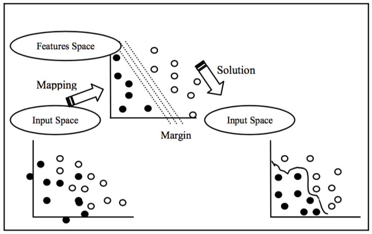
3.2. Support Vector Machines (SVM)

In this study, first implemented classification algorithm is Support Vector Machines (SVM). SVM is a popular and widely used classification algorithm in biomedical studies [13]. SVM basically seperates two different classes of inputs each represented in multi dimensional feature space by generating a boundary function. In SVM algorithm, the inputs are given as (x₁,y₁), ... , (x_i,y_i), x ε R_f (f: number of features) , y_i e {0,1} (class numbers) and SVM will output a boundary plane seperating each class with the greatest margin. The output boundary plane of the SVM will be as follows:

where w is the normal of the boundary plane seperating two classes, b is bias.

For the representation of different classes, regular breathing episodes are labelled as '0', as not an apnea episode, and pre-apnea episodes are labelled as '1', as an apnea episode. SVM algorithm is implemented by using the machine learning tool-box of MATLAB software. Default parameters and kernels of SVM toolbox of MATLAB are used for the implementation. Figure 9 shows the general idea behind SVM classification algoithm.

3.3. k-Nearest Neighbors (kNN)

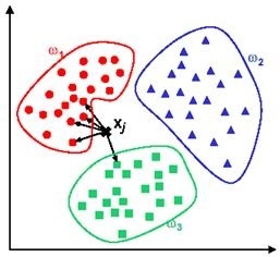
For the 2^nd classification algorithm k-Nearest Neighbors (kNN) is used. kNN simply measures the distance of an input to all of the training dataset points in multi dimensional feature space. Then, the test input will be labelled as the class of the closest training point to itself. This approach is known as kNN-1. In another versions of kNN, defined as kNN-t (such as kNN-3, kNN-5 etc.), the closest t points to the test sample are detected and then a voting mechanism decides the class of the input. Consider a test sample that we would like to predict whether it is a pre-apnea segment. If two out of three closest points to the test sample belong to pre-apnea class, then this test input will be assigned to pre-apnea class as a result of 2-1 voting. In figure 10, an example of kNN-5 is given. For a new test input given to the system, closest 5 points are determined. 4 out of these closest 5 points belong to class w₁ and the remaining data point is in class w₃. The output of the system will be class w₁ as a result of 4-1 voting.

3.4. Linear Regression Approach for Classification (LR)

Linear Regression (LR) basically is a regression algorithm where the output is a real number, not a class. In this study, we approach this classification problem as regression. Similar to SVM learning, in training set pre-apnea episodes are labelled as '1' and regular breathing will be '0'. LR output will be a real number not only 0 or 1. In order to assign the test sample to a class, we should decide a level, call it l. The output higher than l value will be labelled as '1', and if the output is lower than l, then it will be assigned to class '0'.

3.5. Feature Reduction by RANSAC

Selected 39 features are used for classification of a signal interval as pre-apnea or not. However, it is possible to decrease the dimension of the feature space and improve the classification accuracy by eliminating some of the irrelevant features. For this purpose, Randomly Select and Compute (RANSAC) algorithm is used. First, the accuracy of the classification is calculated by using all 39 features. Results are shown in Results & Discussion section. Then, 35 features out of 39 are randomly selected and accuracy is calculated using these 35 features. RANSAC algorithm is implemented for 1000 repetitions and features are noted having highest accuracy in classification. Similar feature reduction algorithm is computed for 30, 25, 20 features. Results suggest that randomly selected 30 features have the best performance in prediction of OSA episodes and further reduction of features also diminishes the performance. Feature reduction and classification algorithm is as follows:

Choose number of features (Repeat for n=35,30,25 and 20) randomly select n features (Repeat for 1000 times)

• train and classify by selected learning algorithm
• record features giving highest accuracy in selected learning algorithm
• 5-fold cross validation for accuracy, sensitivity, specificity

3.6. Entropy Based Feature Reduction

Entropy is used as a different measure to reduce feature numbers in learning process. Entropy is a probability measure in log scale representing total probability of all labels, in this study "1" or "0". The entropy equation is given as follows:

where p is the probability and i represents the classes (pre-apnea or regular breathing).

The entropy of all 39 features is calculated and the features having the lowest entropy values are eliminated and not used in training or testing. The calculated values of all features are independently normalized and mapped to either "0" or "1" by comparing with the mean value of the corresponding feature.

3.7. Performance Measures

Performance measures are calculated using 5-fold cross validation. The whole data set is randomly divided into two categories: training set, test set. Training set contains 80% of the data set, and learning algorithm is trained by these input instances. The remaining 20% is used for classification and measuring the accuracy, sensitivity and specificity of the proposed approach. The training process repeated for 5 times and in each repetition, a new 80% training set is generated. After training and classifying the signals 5 times, the mean values are noted as final performance measures. True Positive (TP) is that system predicted pre-apnea ('1') segment as in truth the segment is labelled as pre-apnea. True Negative (TN) is that the output of the prediction is regular breathing ('0' or not pre-apnea), when the corresponding episode is actually regular breathing. False Positive (FP) is the case that system gives an output of pre-apnea episode ('1') as it should be regular breathing (false alarm) and for False Negative (FN), system will decide a segment as regular breathing however, the patient is actually about to face apnea in a short period of time (miss to warn pre-apnea). Using the definitions accuracy, sensitivity and specificity is calculated in the results section. Accuracy is the correct prediction of a pre-apnea interval (labelled '1') or regular breathing interval (labelled '0').

Sensitivity is the correct classification ratio of pre-apnea intervals (labelled '1') when the corresponding episode is actually pre-apnea.

Similarly specificity is the ratio of correct classification of regular breathing intervals (labelled '0') if regular breathing episodes are given as input to the system.

4. Results & Discussion

The performance of the proposed prediction algorithm is measured in terms of accuracy, sensitivity, specificity, accuracy for SVM, kNN & LR. Primarily, extracted 39 features are used for learning and classification process. 62% of accuracy for SVM is recorded which is below accepted levels. Followingly, feature reduction approach is used and performance is measured for using different features. Table 1 shows the performance measures of prediction methods for the given parameters.

Table 1. Performance measure of SVM for features reduced by RANSAC and Entropy based method.

SVM with RANSAC - Entropy
Number of Features	Accuracy	Sensitivity	Specificity
39	0.625-0.625	0.884-0.884	0.546-0.546
35	0.843-0.783	0.890-0.811	0.802-0.766
30	0.869-0.805	0.906-0.820	0.763-0.788
25	0.858-0.762	0.915-0.743	0.720-0.775
20	0.824-0.772	0.908-0.818	0.750-0.734

Table 2. Performance measure of kNN-3 for features reduced by RANSAC and Entropy based method.

kNN-3 with RANSAC - Entropy
Number of Features	Accuracy	Sensitivity	Specificity
39	0.624-0.646	0.605-0.631	0.647-0.665
35	0.649-0.688	0.663-0.702	0.630-0.671
30	0.706-0.724	0.748-0.766	0.682-0.692
25	0.694-0.686	0.708-0.654	0.683-701
20	0.710-0.643	0.692-0.665	0.722-0.617

Table 3. Performance measure of kNN-5 for features reduced by RANSAC and Entropy based method.

kNN-5 RANSAC - Entropy
Number of Features	Accuracy	Sensitivity	Specificity
39	0.765-0.780	0.782-0.805	0.744-0.768
35	0.810-0.832	0.823-0.814	0.800-0.845
30	0.826-0.810	0.835-0.784	0.813-0.832
25	0.814-0.776	0.820-0.758	0.796-0.790
20	0.763-0.724	0.785-0.742	0.757-0.706

Table 4. Performance measure of LR for threshold l=0.2 for features reduced by RANSAC and Entropy based method.

kNN-5 RANSAC - Entropy
Number of Features	Accuracy	Sensitivity	Specificity
39	0.706-0.653	0.744-0.688	0.689-0.620
35	0.723-0.605	0.752-0.586	0.705-0.614
30	0.756-0.624	0.744-0.645	0.782-0.596
25	0.695-0.630	0.714-0.646	0.684-0.622
20	0.712-0.616	0.683-0.597	0.734-0.630

As Table 1 states, for SVM overall performance of all parameters shows improvement after a few features are reduced. Elimination of unrelated features to the apnea prediction, increases prediction accuracy. However, further feature reduction has unfavorable effect on accuracy and the optimal results are obtained for set containing 30 features. Eliminated features are analyzed, and it is noticed that following features are always discarded in reduction process:

• maximum time between peak of inspiration and average value
• maximum time between peak of expiration and average value
• minimum time between average value and peak of expiration
• minimum time between average value and peak of inspiration
• ratio of time that respiratory signal is above the average value to the time respiratory signal is below the average value

We can comment that some of the features representing minimum or maximum time recorded for inspiration or expiration are generally eliminated in feature reduction. Thus, it can be concluded that extreme (minimum or maximum time) inspiration & expiration durations are not significant to predict OSA. Features providing information on general respiratory structure like mean values inspiration/expiration or magnitude of nasal airflow signal are more crucial and needed to be analysed especially.

SVM has the best prediction performance in accuracy, sensitivity, overall and kNN has the highest specificity rate. kNN-1 & kNN-7 are also tested for the selected features, however accuracy is lower than 0.5 and results are not added in the table since it does not show any significant meaning.

Results do not show much significant difference between two feature reduction methods. Both methods may show higher performance depending on the features used and the corresponding classification algorithms. However, it is noticeable that entropy approach fails if the amount of excluded features are increased. Therefore, we can comment that eliminating features, which have very low entropy, improves the classification performance. On the other hand, further feature reduction may cause accuracy degradation.

5. Conclusion

In an overnight sleep, OSA patients may face apnea more than 300 times. In addition to decrease in sleep quality and inability to maintain resting during sleep, OSA can be associated with other disorders like hypertension, stroke. It is an underestimated critical disorder, which BPAP or CPAP devices are used to overcome apnea. CPAP devices might be hard for some patients to tolerate at higher pressures. Besides, it may not be an influential treatment for people with extreme OSA. On the other hand, BPAP devices are more appropriate for people originally diagnosed with OSA. Having a sleep with these type of devices, discomforts the patients for both. To overcome these disadvantages of these devices and warn the patient before an apnea epsiode, an early warning algorithm that predicts OSA episodes is proposed in this study. The accuracy of apnea prediction is over 87% with a sensitivity of 91% when SVM is used. kNN approach has lowest accuracy but in return of highest specificity slightly above 0.8. For LR as a classification algorithm method, proper classification boundary selection (l value) significantly effects the general accuracy however, still it did not present any satisfactory results in any of the performance measures. 76% of specificity value of SVM suggests that there may be some cases, the algorithm labels a nasal airflow period as pre-apnea where actually it is not. Studies generally focus on detecting apnea during sleep to improve the performance of BiPAP devices. Also there are some studies that researchers try to predict OSA patients in diagnosis stage. We approached the OSA problem in a different way. The novelty of this study is that findings are fundamental to develop an early predicting warning system before patient faces an OSA episode. Enhanced accuracy, sensitivity, specificity may contribute to the development of these devices. Total computational time of the algorithm for a single 1 minute nasal airflow signal is less than 0.3 seconds. Thus, it may be useful and comfortable approach that a device, records the nasal airflow signal of the patient throughout the night and runs the proposed algorithm in real-time. By this way we may be able to warn or wake the patient up before his/her respiration fails. In future studies, specificity ratio will be tried to be improved. Development of a hybrid learning tool, combining the high accuracy, sensitivity performance of SVM and high specificity of kNN, will significantly improve the prediction of OSA segments.

References

[1] F. Roche, V. Pichot, E. Sforza, I. Court-Fortune, D. Duverney, F. Costes, M. Garet and J.-C. Barthe Lemy, "Predicting sleep apnea syndrome from heart period: a time-frequency wavelet analysis," European Respiratory Journal, vol. 22, pp. 937-942, 2003. View Article
[2] P. E. Peppard, T. Young, J. H. Barnet, M. Palta, E. W. Hagen and K. M. Hla, "Increased prevalence of sleep-disordered breathing in adults," Am. J. Epidemiol., vol. 177, no. 9, pp. 1006-1014, 2013. View Article
[3] M. R. Mannarino, F. Di Filippo and M. Pirro, "Obstructive sleep apnea syndrome," Eur. J. Intern. Med., vol. 23, no. 7, pp. 586-593, 2012. View Article
[4] C. A. Kushida, M. R. Littner, T. Morgenthaler, C. A. Alessi, D. Bailey, J. J. Coleman, L. Friedman, M. Hirshkowitz, S. Kapen, M. Kramer, T. Lee-Chiong, D. L. Loube, J. Owens, J. P. Pancer and M. Wise, "Practice parameters for the indications for polysomnography and related procedures: an update for 2005," Sleep, vol. 28, no. 4, pp. 499-521, 2005. View Article
[5] S. M. C. o. W. N. York, "Obstructive Sleep Apnea," 2010. [Online]. Available: http://www.sleepmedicinecenters.com/SleepDisorders/ObstructiveSleepAnea. [Accessed 12 May 2016]. View Article
[6] R. Nowak, T. Corbridge and B. Brenner, "Noninvasive Ventilation," in Proceedings of the American Thoracic Society, 2009. View Article
[7] L. Chen, X. Zhang and C. Song, "An Automatic Screening Approach for Obstructive Sleep Apnea Diagnosis Based on Single-Lead Electrocardiogram," IEEE Trans. Autom. Sci. Eng., vol. 12, no. 1, pp. 106-115, 2015. View Article
[8] T. C. Huang, H. Y. Chen and W. C. Fang, "Real-Time Obstructive Sleep Apnea Detection Based on ECG Derived Respiration Signal," in IEEE International Symposium on Circuits and Systems (ISCAS), 2012. View Article
[9] J. Han, H. B. Shin, D. U. Jeong and K. S. Park, "Detection of apneic events from single channel nasal airflow using 2nd derivative method," Comput. Method. And Prog. Biomed., vol. 91, pp. 199-207, 2008. View Article
[10] A. Yadollahi and Z. Moussavi, "Acoustic Obstructive Sleep Apnea Detection," in Engineering in Medicine and Biology Society (EMBC), 31st Annual International Conference of the IEEE, 2009. View Article
[11] M. S. Kim, Y. C. Cho, S. Seo, C. Son and Y. Kim, "Comparison of Heart Rate Variability (HRV) and Nasal Pressure in Obstructive Sleep Apnea (OSA) Patients During Sleep Apnea," Measurement, vol. 45, no. 5, pp. 993-1000, 2012. View Article
[12] S. I. Rathnayake, I. A. Wood, U. R. Abeyratne and C. Hukins, "Nonlinear features for single-channel diagnosis of sleep-disordered breathing diseases," IEEE Trans. Biomed. Eng., vol. 57, no. 8, pp. 1973-1981, 2010. View Article
[13] M. M. Nano, X. Long, J. Werth, R. M. Aarts and R. Heusdens, "Sleep Apnea Detection Using Time-Delayed Heart Rate Variability," in Engineering in Medicine and Biology Society (EMBC), 37th Annual International Conference of the IEEE, 2015. View Article
[14] L. Almazaydeh, K. Elleithy and M. Faezipour, "Obstructive Sleep Apnea Detection Using SVM-Based Classification of ECG Signal Features," in IEEE International Conference on Electro/Information Technology (EIT), 2012. View Article
[15] O. C. Celebi, "Celebi Tutorial: Neural Networks and Pattern Recognition Using MATLAB," [Online]. Available: http://www.byclb.com/TR/Tutorials/neural_networks/ch11_1.htm. View Article